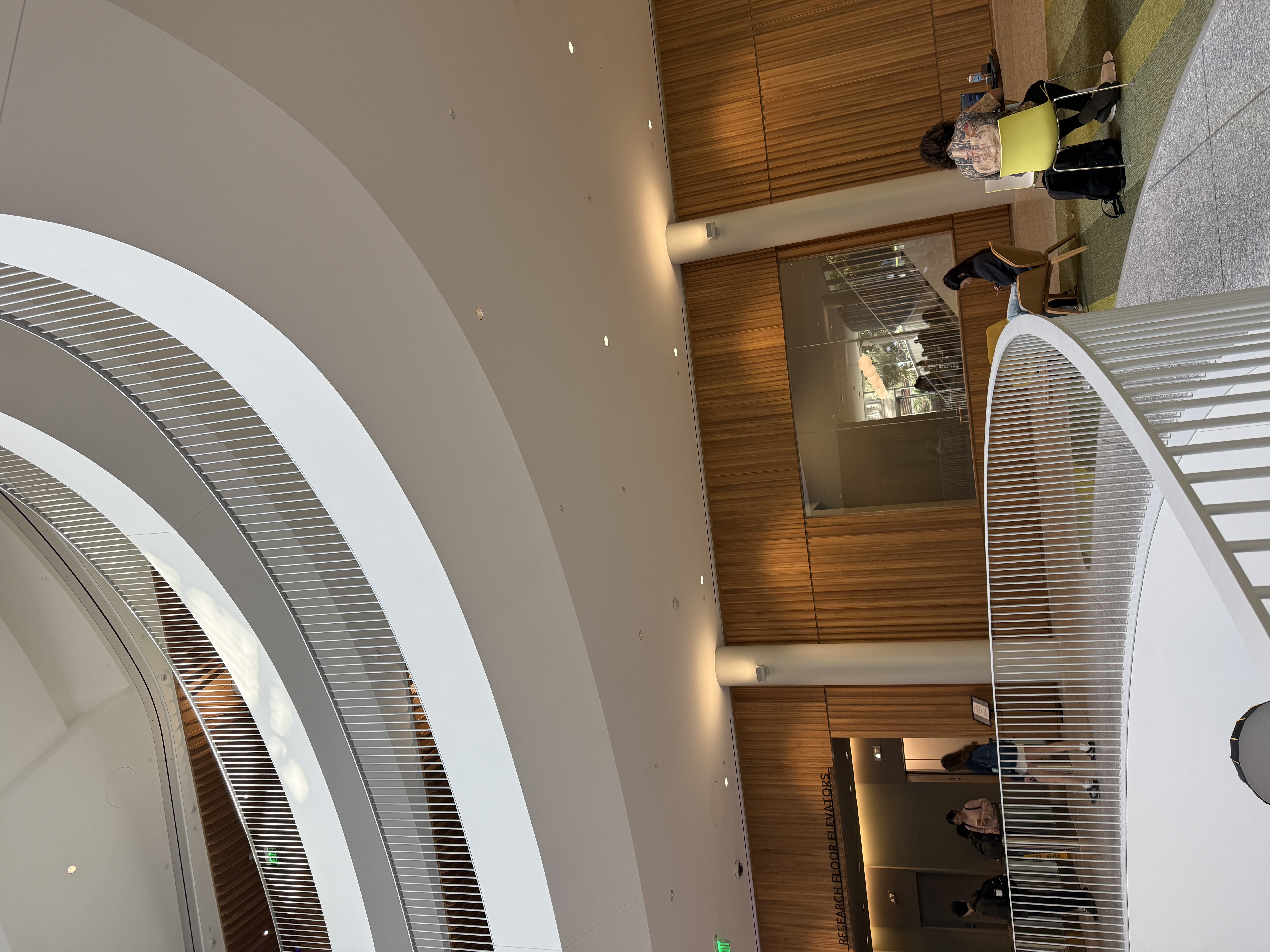
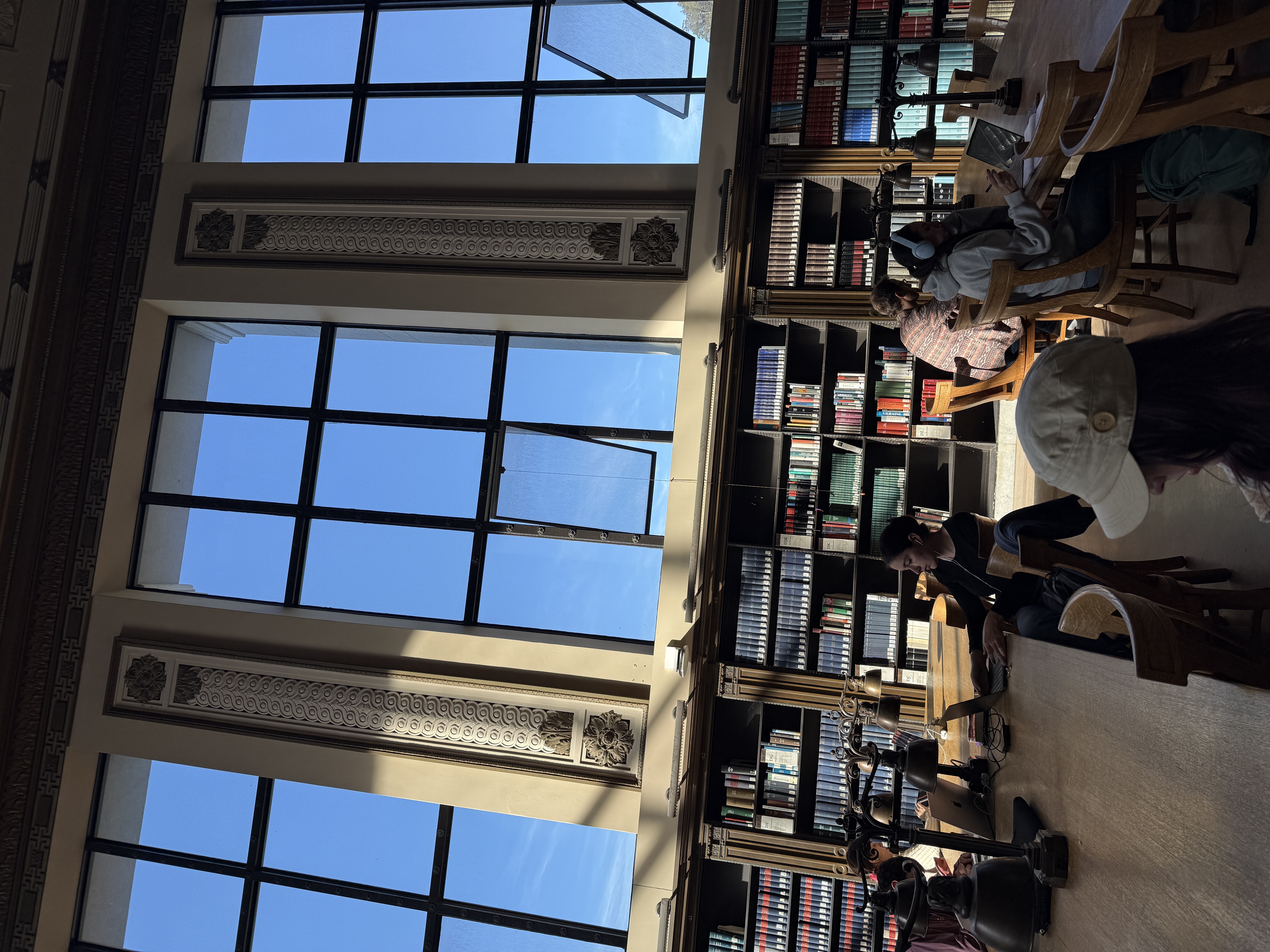
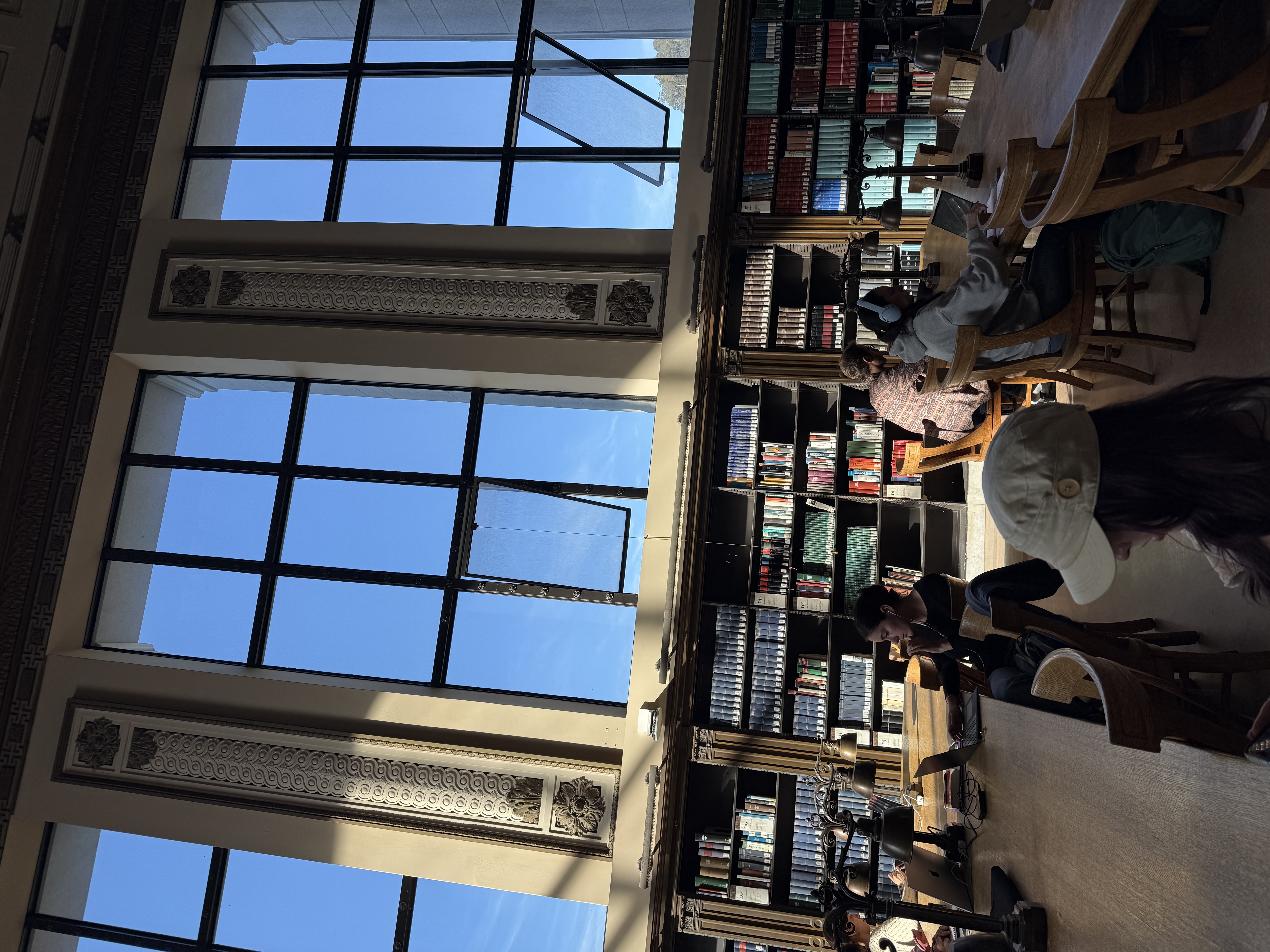
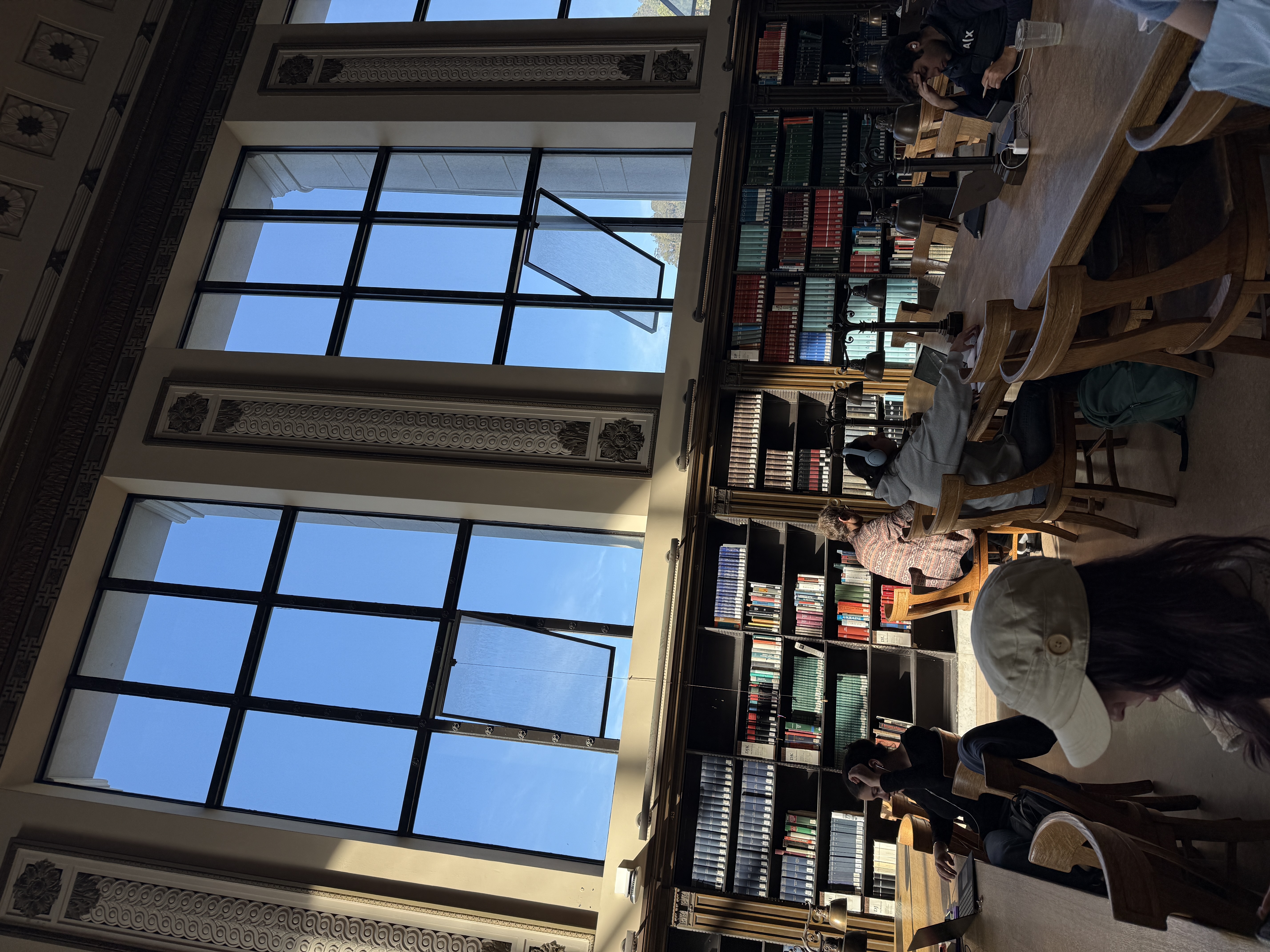
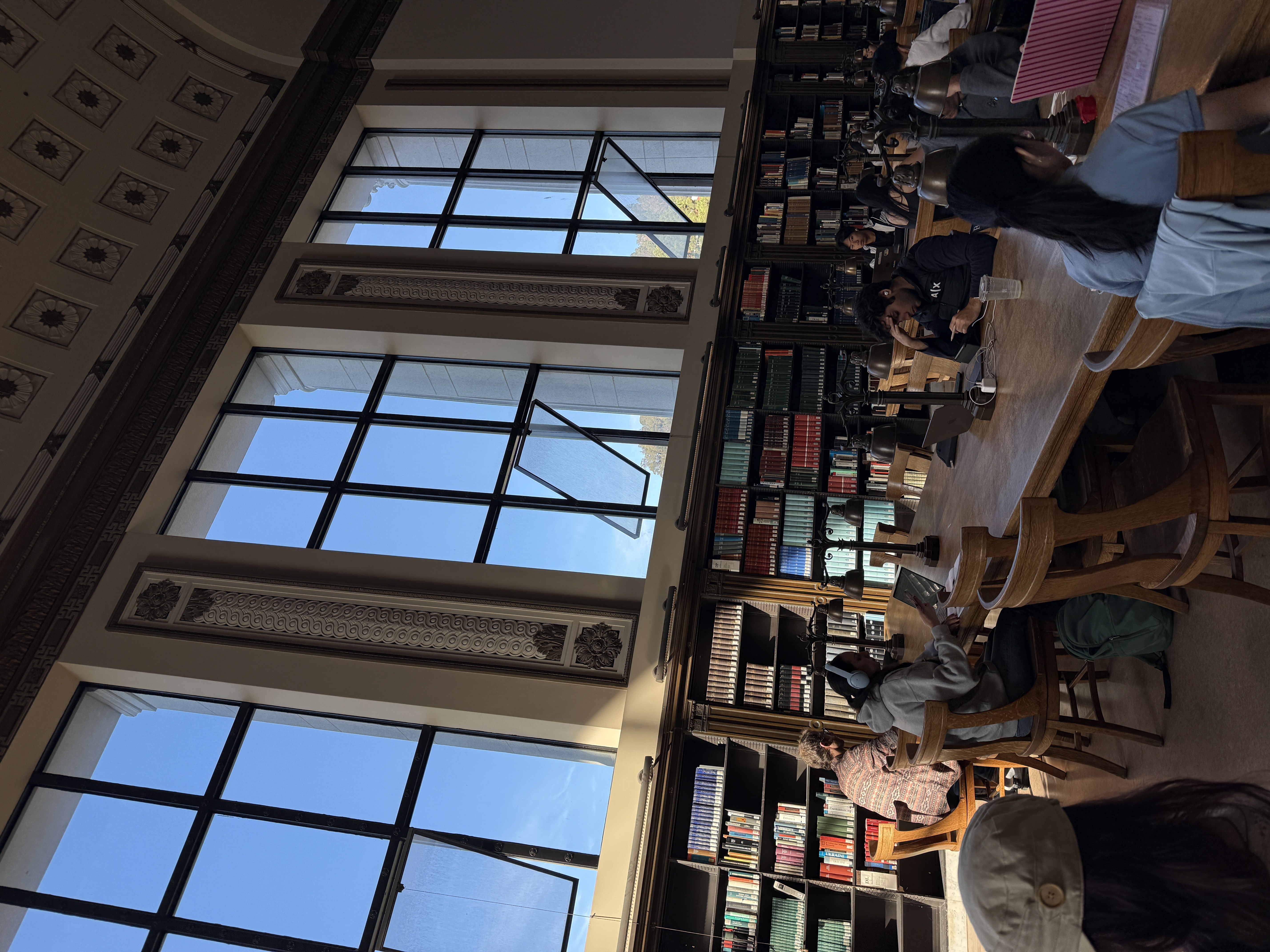
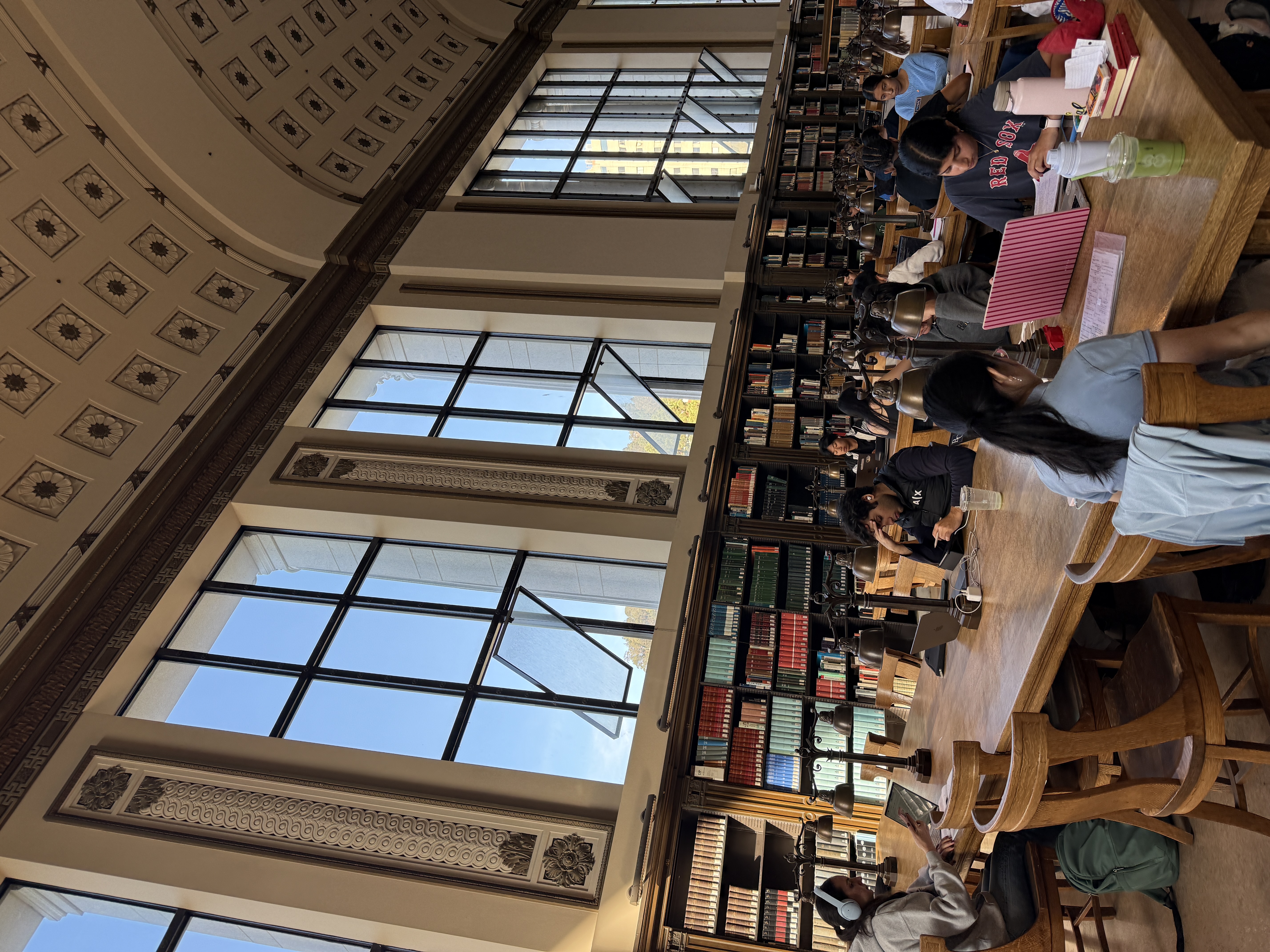
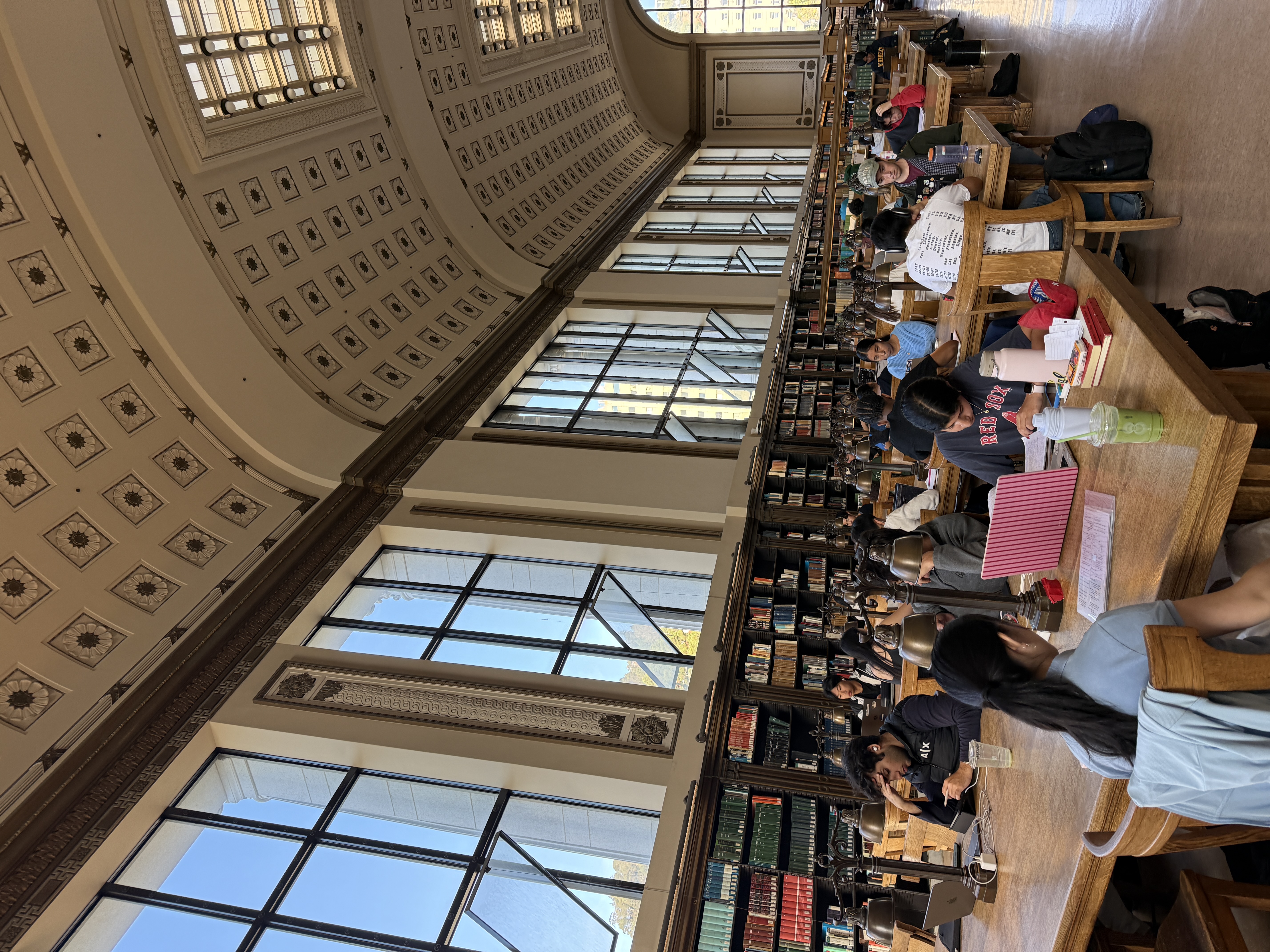
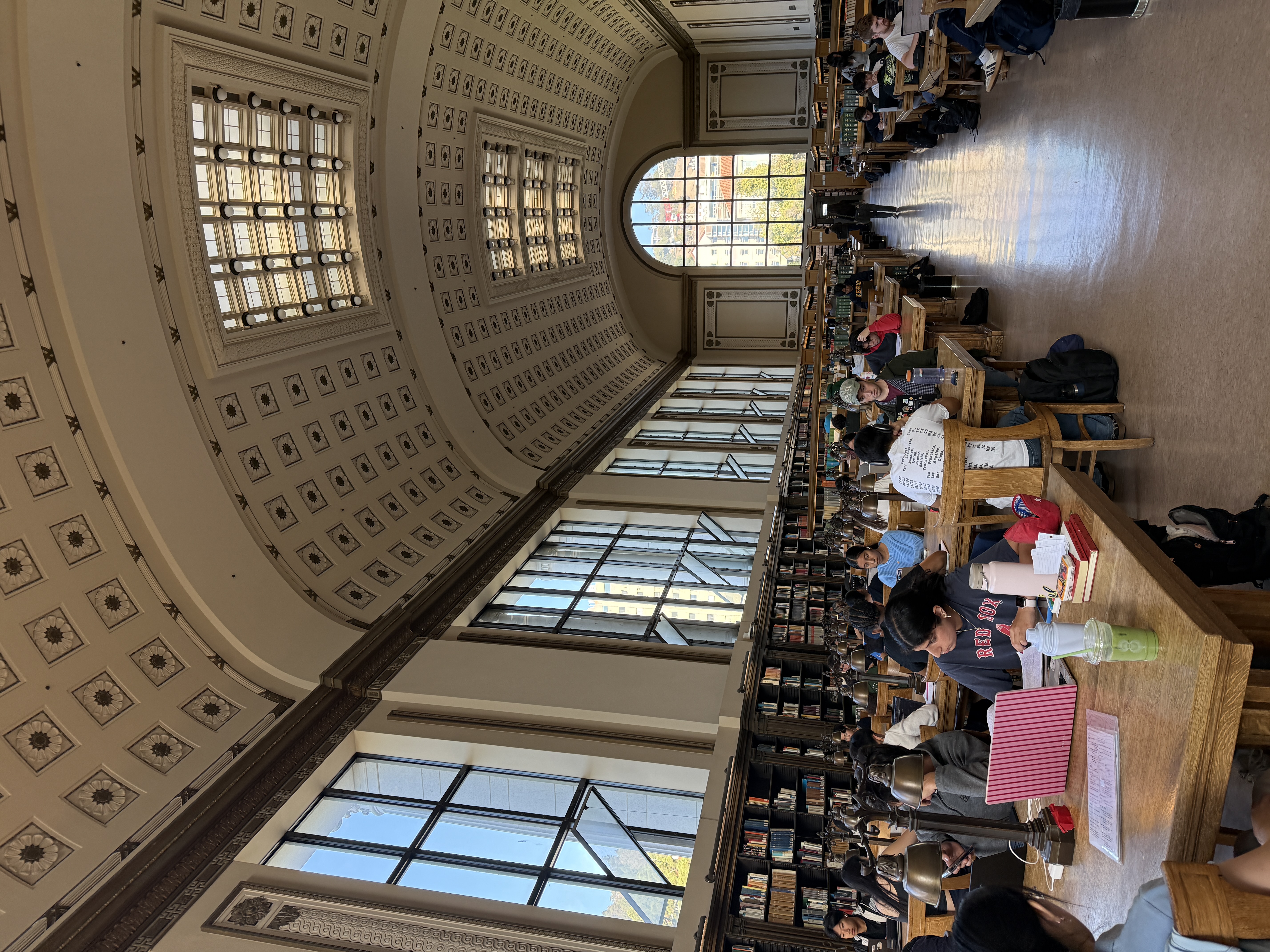
Homographies are used to map points between images. This is accomplished with a 3x3 matrix that maps a point in one image (x, y), to its corresponding point in another image (x', y'). The bottom two equations are used to solve for the (x', y') values.
    [x  y  1  0  0  0  -x*x'  -y*x'] h = x'
    [0  0  0  x  y  1  -x*y'  -y*y'] h = y'
After getting the (x', y') values, the homography matrix is solved for by stacking the rows for all points gives a system Ah = b. After that, I selected 7-10 points in each image pair that correspond to each other.
The blue dots are the manually clicked points, and the red x's are the other image's points mapped through the homography matrix.
First 4 rows of the system
    [657.1  238.7  1    0      0     0   -311320.5  -113096.2] h = 473.8
    [  0      0    0  657.1  238.7   1   -157661.8   -57275.2] h = 239.9
    [344.5  496.8  1    0      0     0    -48924.6   -70565.2] h = 142.0
    [  0      0    0  344.5  496.8   1   -164373.2  -237079.9] h = 477.2
    ...
Recovered H:
    [[ 1.3389     0.0117    -306.50 ]
     [ 0.2315     1.2291    -153.88 ]
     [ 0.000317   0.000031     1    ]]
Mean reprojection error: 2.1 px.
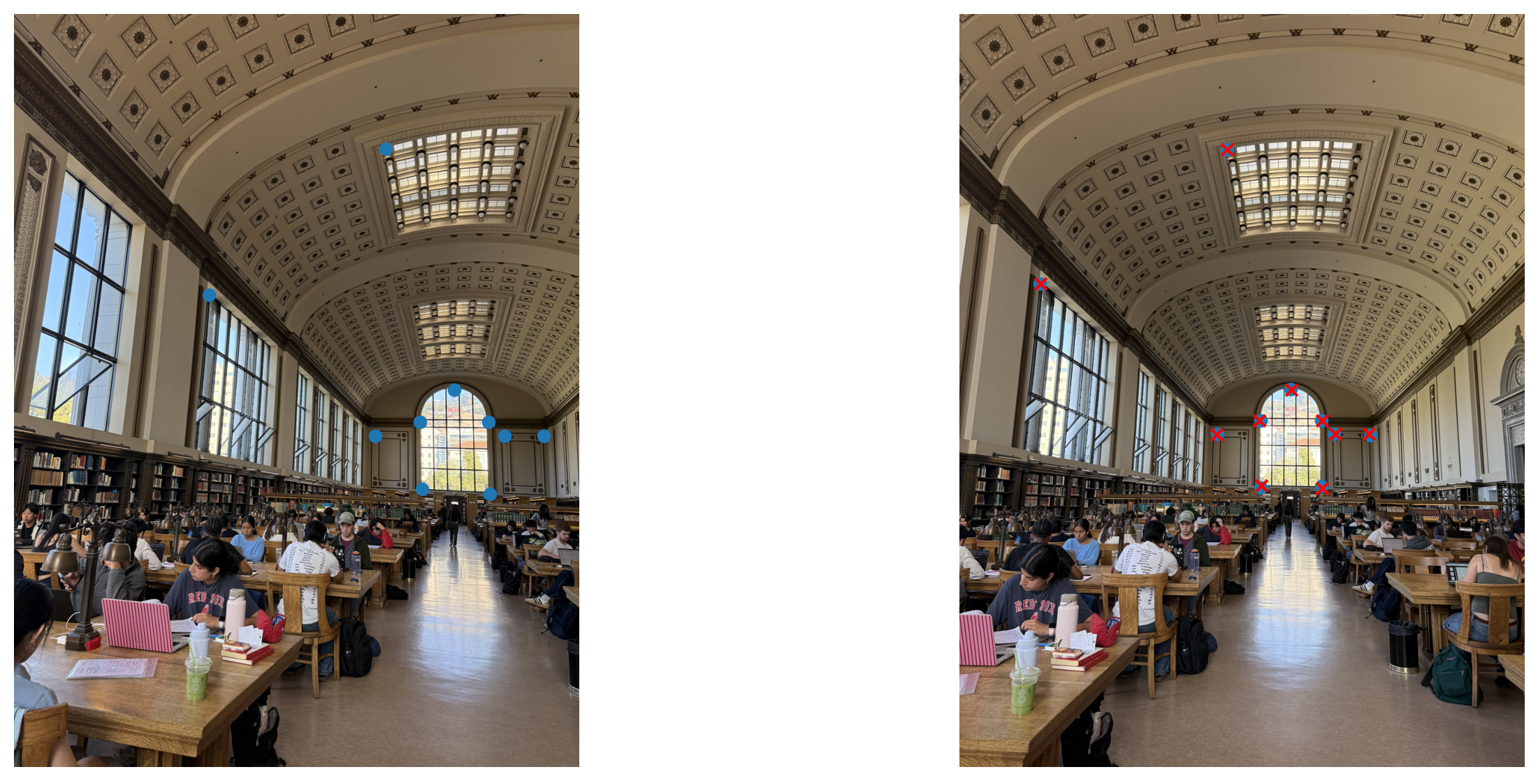
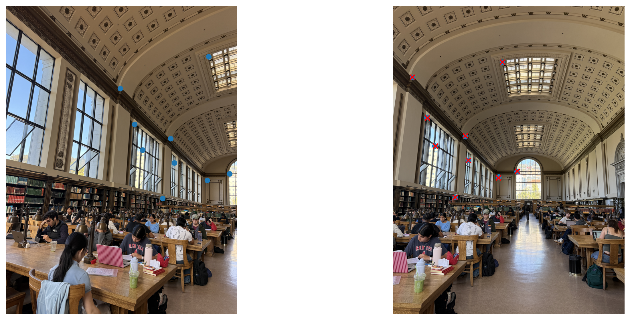
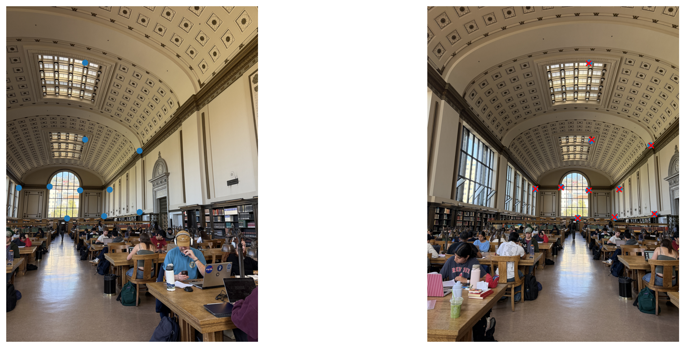
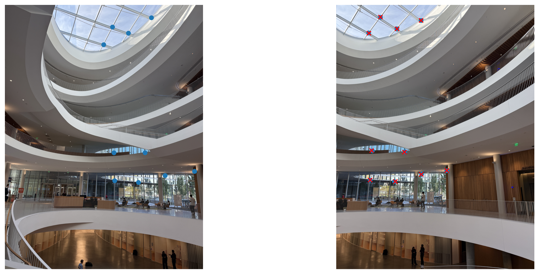
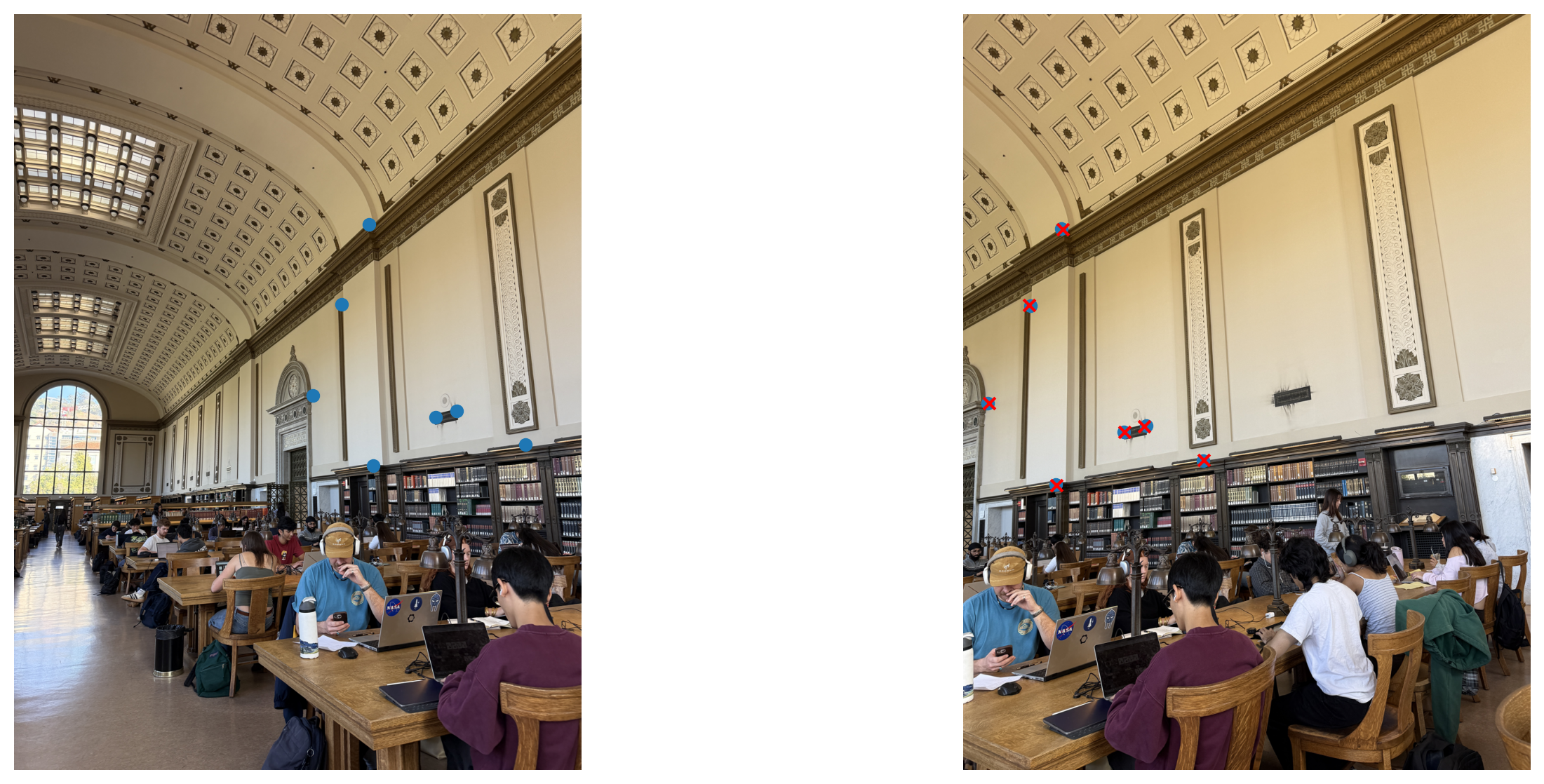
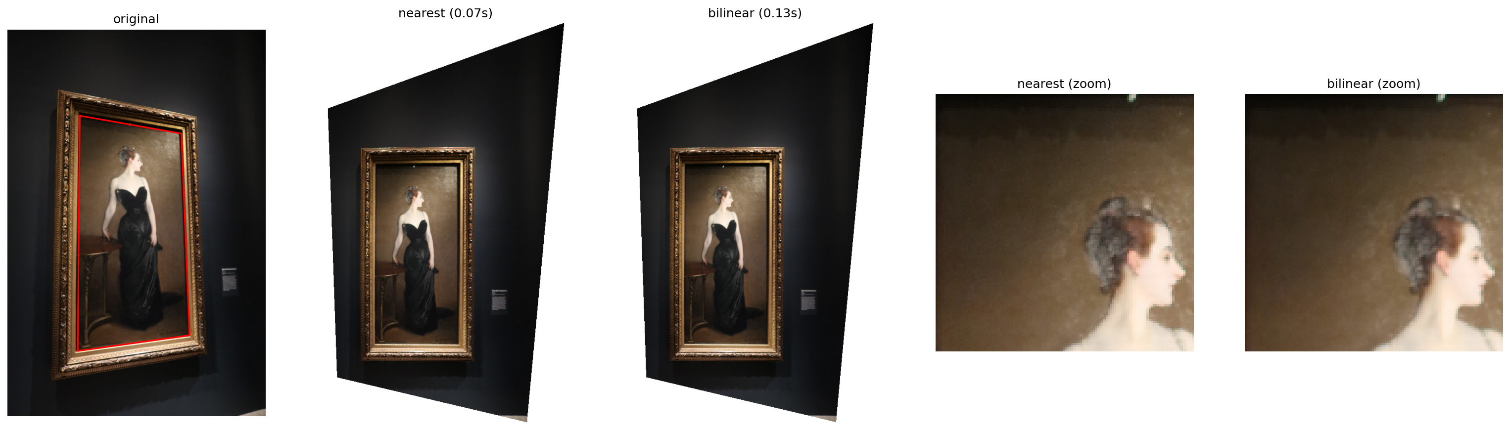
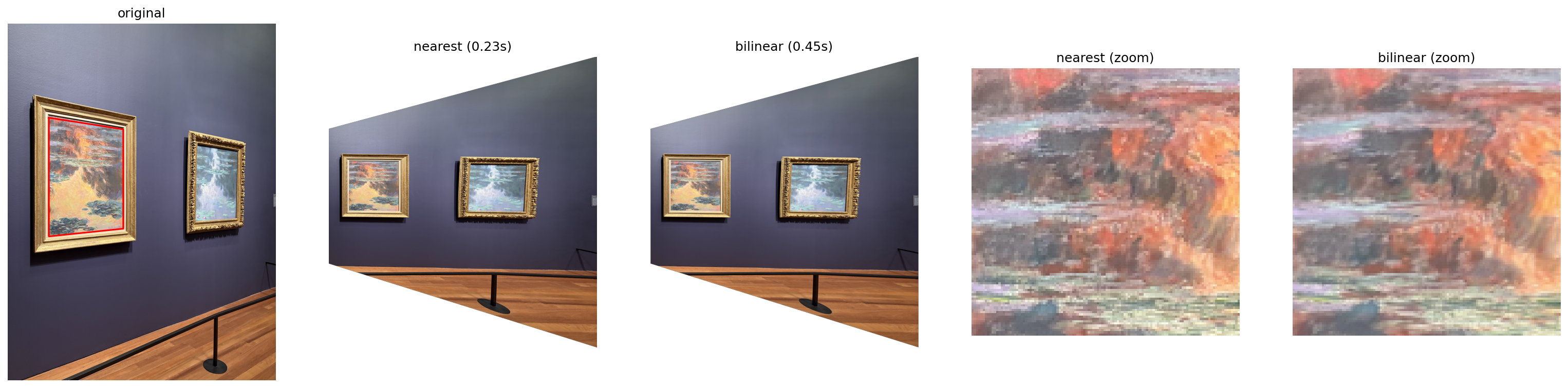
Image warping means transforming one image to another image's perspective using homography. Interpolation is the process of estimating a color value between two pixels. When warping an image, the output pixel is the result of interpolation of the input pixels. This can be accomplished using nearest neighbor or bilinear interpolation For nearest neighbor interpolation, you round the coordinates to the nearest pixel value (closest integer for the x and y coordinates). For bilinear interpoation, you take a weighted average of the 4 surrounding pixels, weighted by their distance to the output pixel. In the below examples, we tried bilinear and nearest neighbor interpolation on The Portrait of Madame X and two of Monet's water lilies. The photos of the paintings were taken at an angle, and after clicking on the top left, top right, bottom left, and bottom right corners of each painting, we were able to warp the images to a rectangle with a straight on perspective. The color quality when transferred from the original image to the warped images is quite similar, although the bilinear interpolation results are a bit blurrier. However, the bilinear interpolation was a bit slower than the nearest neighbor interpolation. Both methods did not do super well at preserving the original width of the paintings. The Portrait of Madame X is a bit less wide than the original painting, and the Monet paintings are much wider than their original paintings.
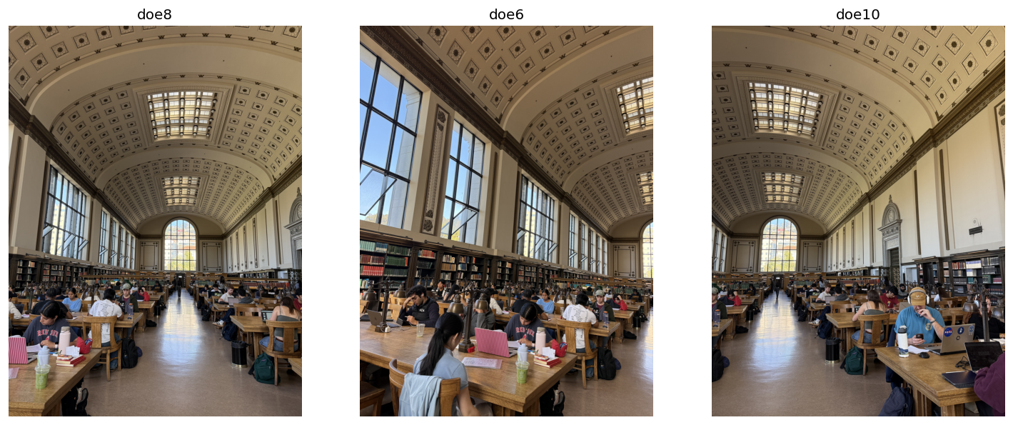
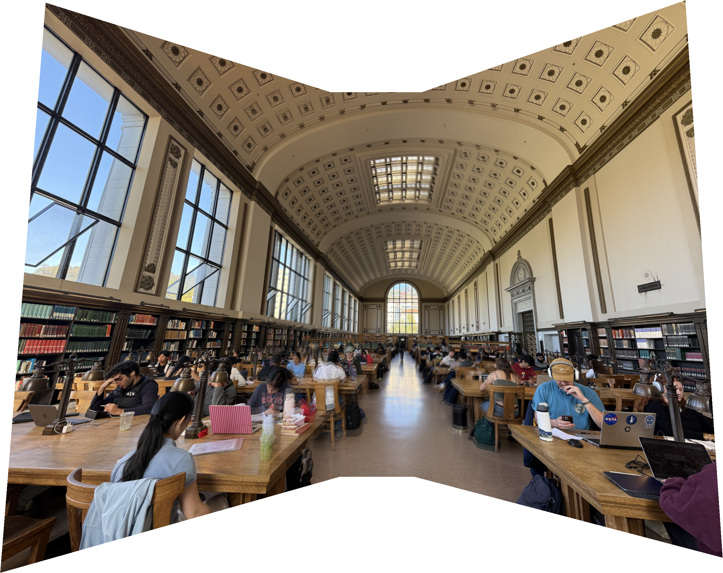
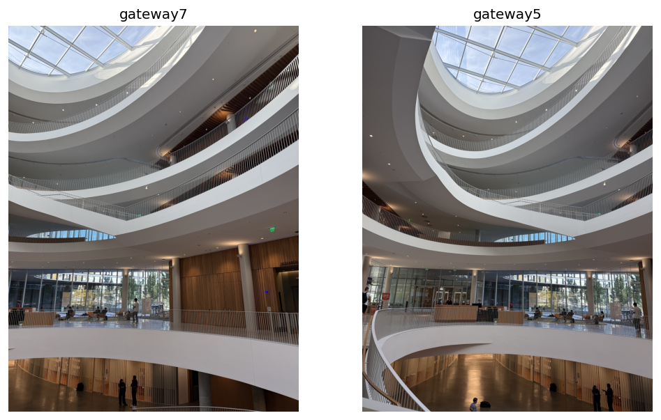
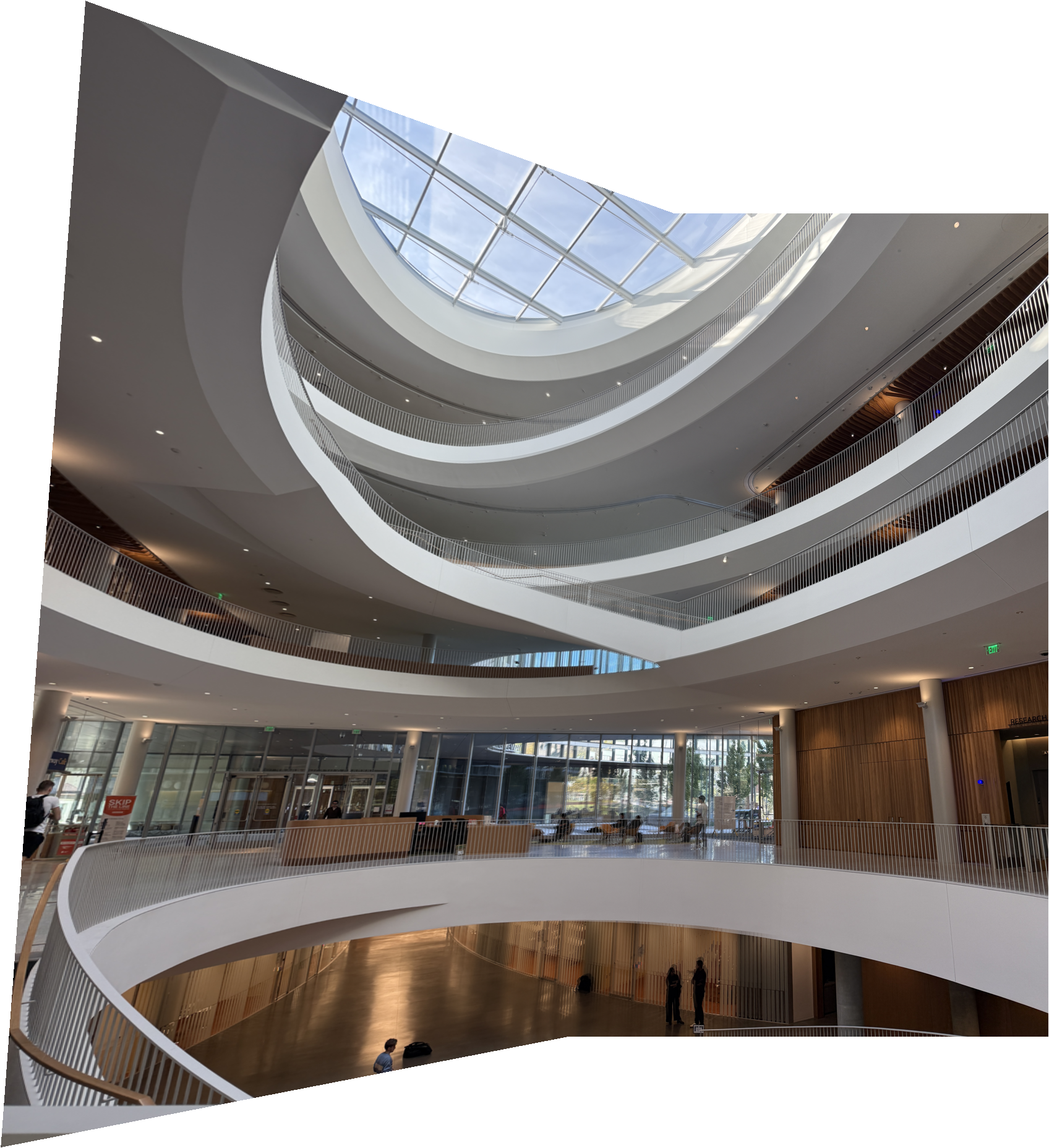
Mosaics consist of multiple images stitched together to create a larger image. For the Mosaics below, I kept the middle photo unwarped and warped the photos to their left and right using homographies from A.2 and bilinear interpolation from A.3. To determine the size of the final mosaic, I mapped the corners of every warped image into the middle image's coordinate system.
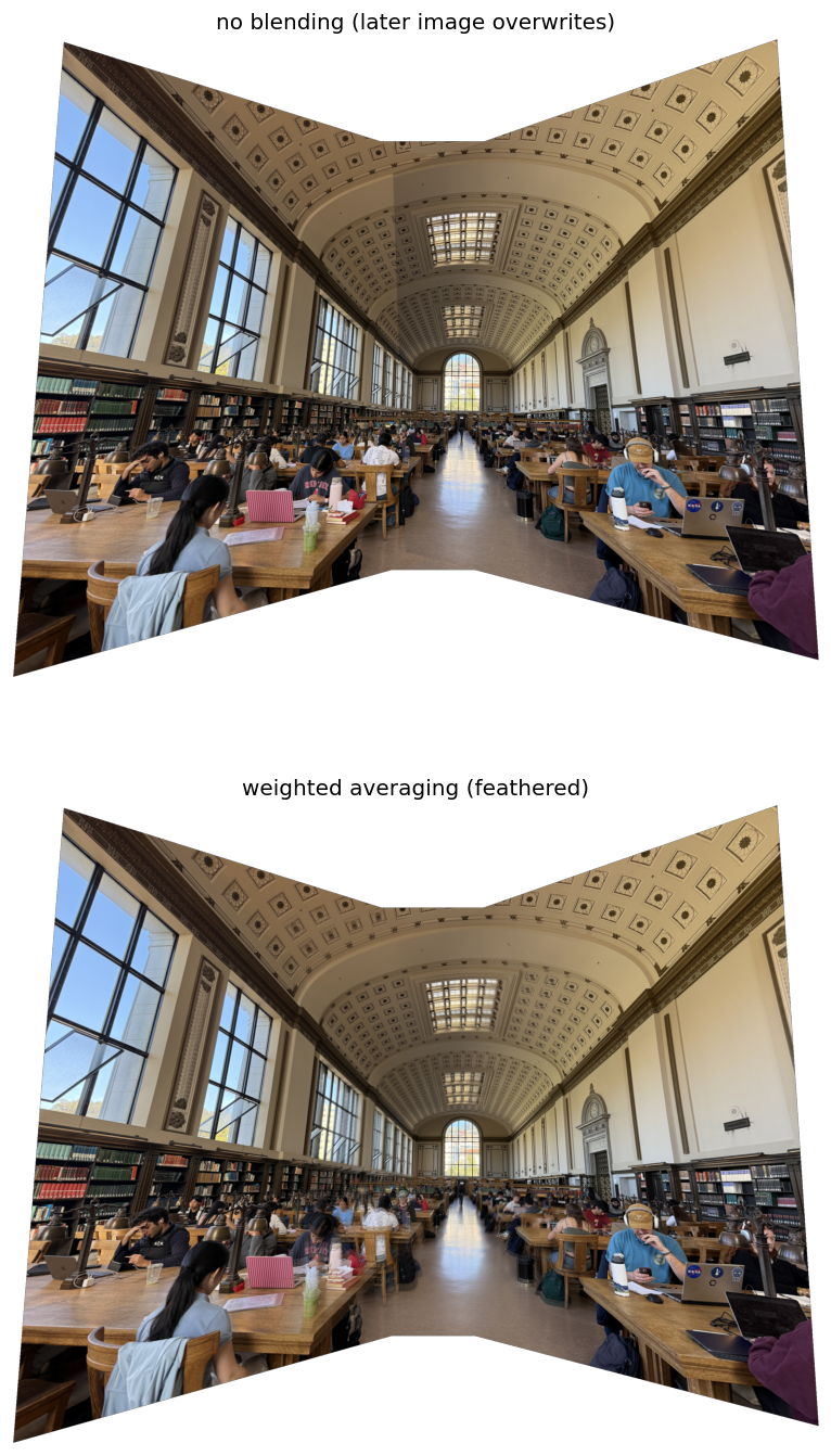
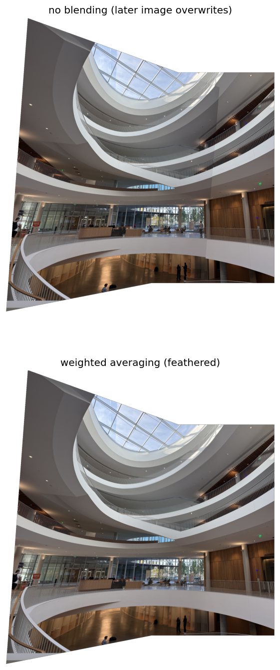
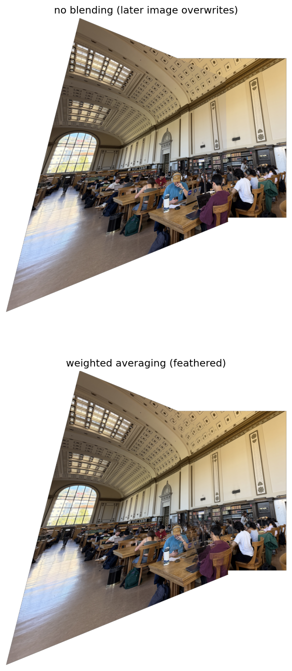
Weighted averaging / feathering is used to blend the images together. Each photo has a weight map that ranges from 1 at the center to 0 at the edges. The weight map is warped with each image so that wherever two images overlap, the output pixel is the weighted average of the two images. Thus, any differences in brightness are blended together. For example, in the first Mosaic below, in the no blending version, the rightside image has a slightly dark left edge that is visible, which the weight map removes. Another failure mode is that the weight map can cause ghosting since some people in the scene slightly moved between the photos.
mosaic = sum(weight_i * image_i) / sum(weight_i)
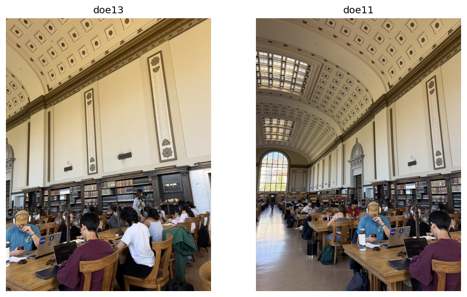
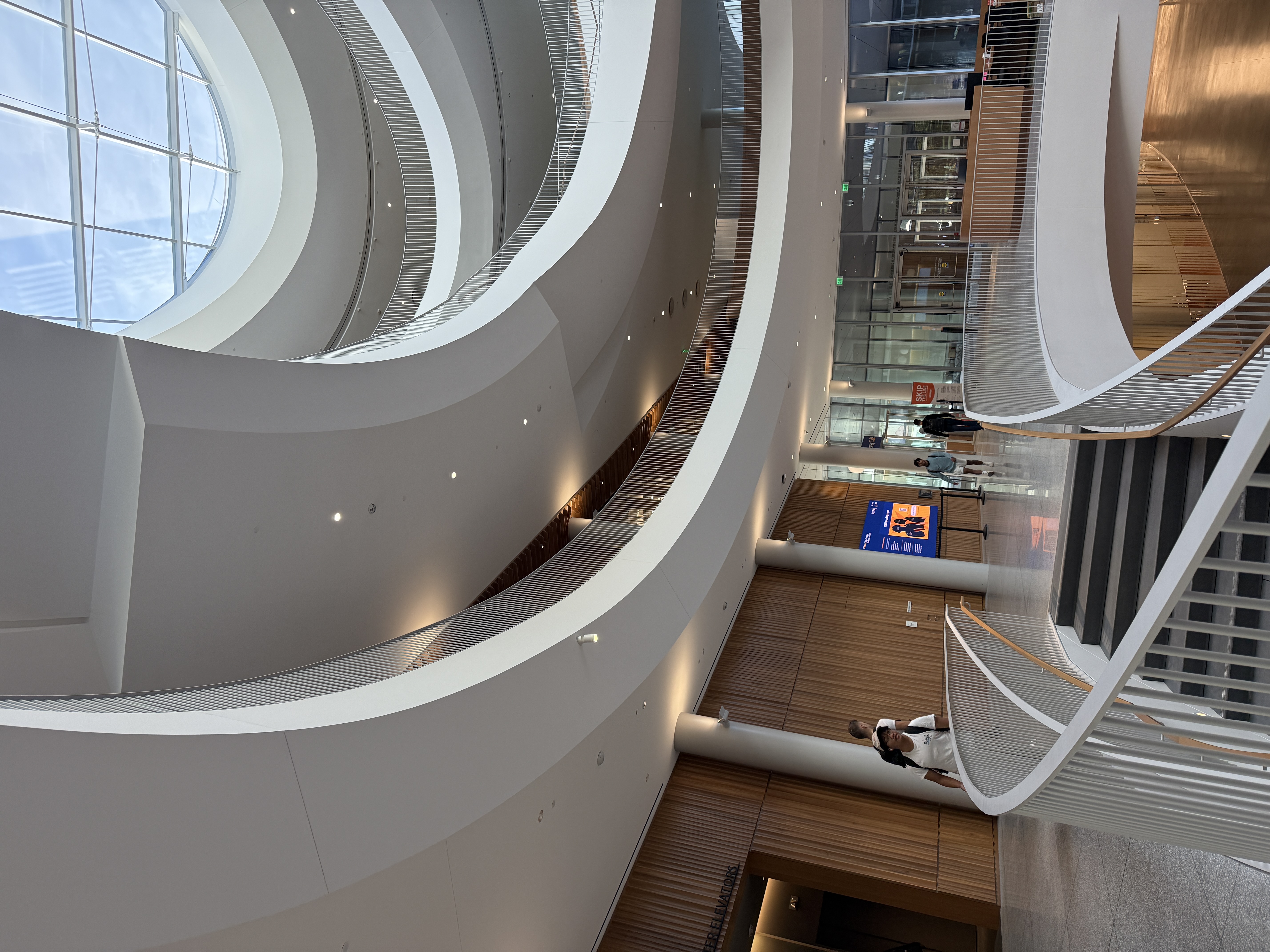
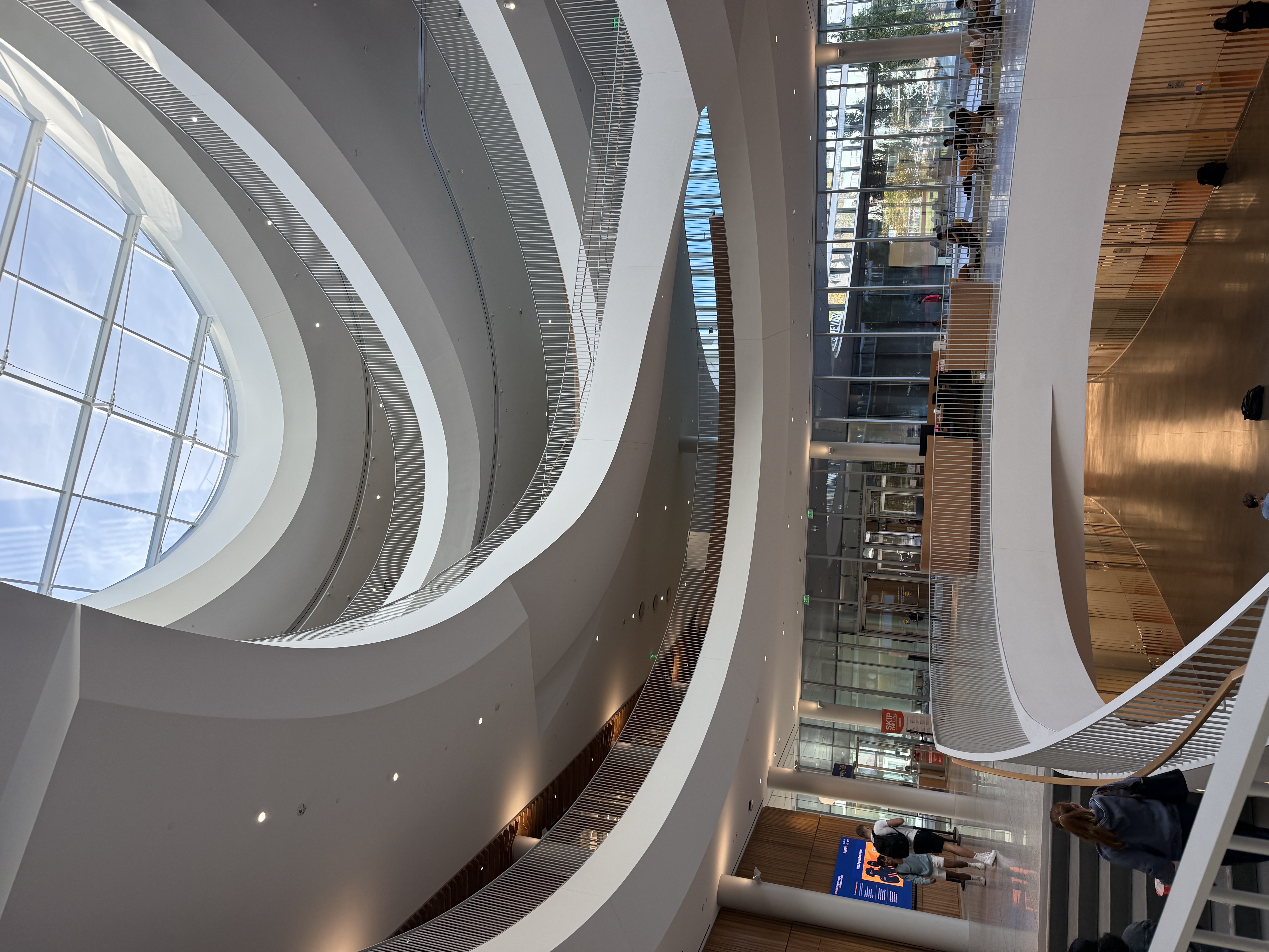
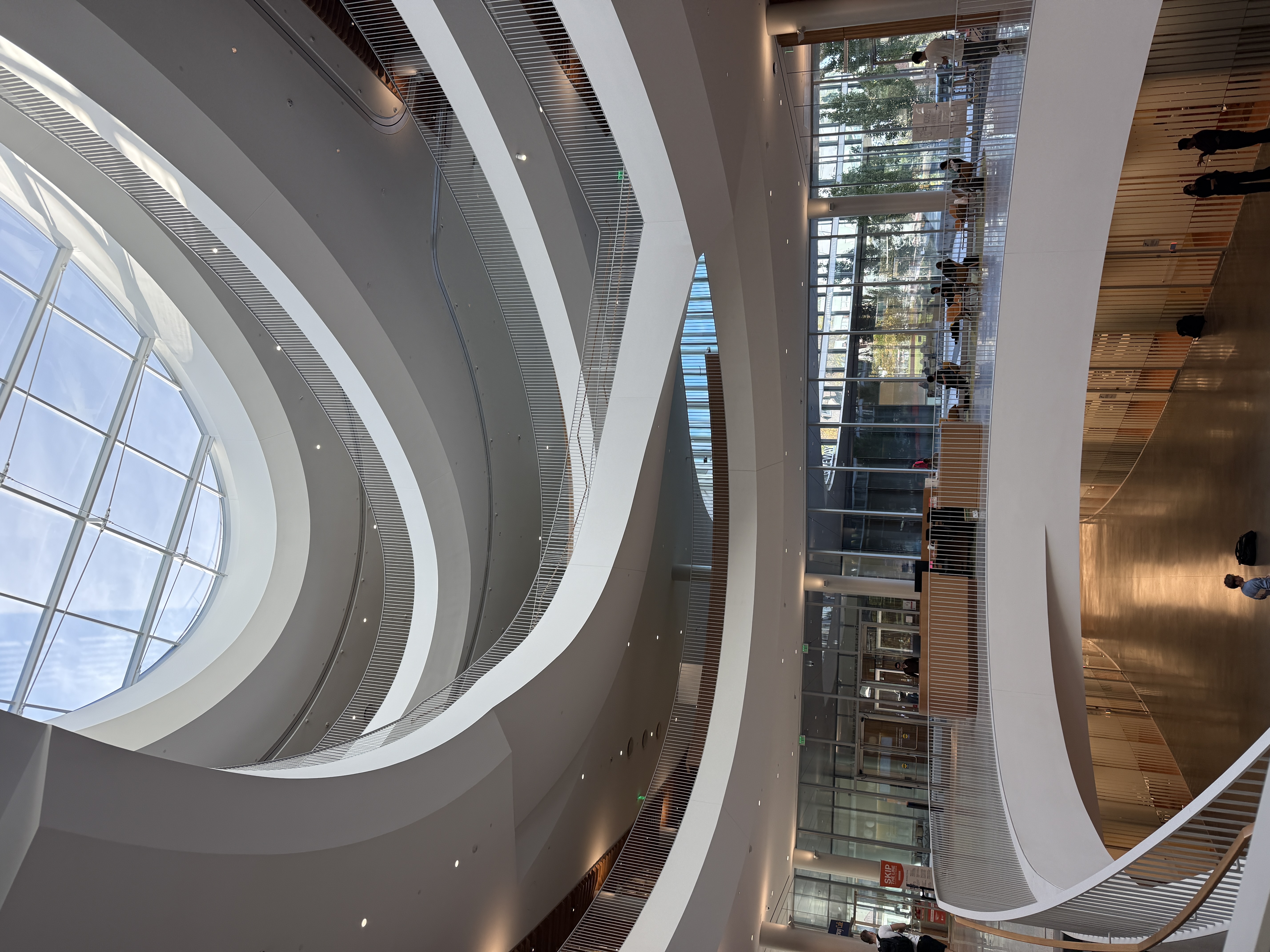
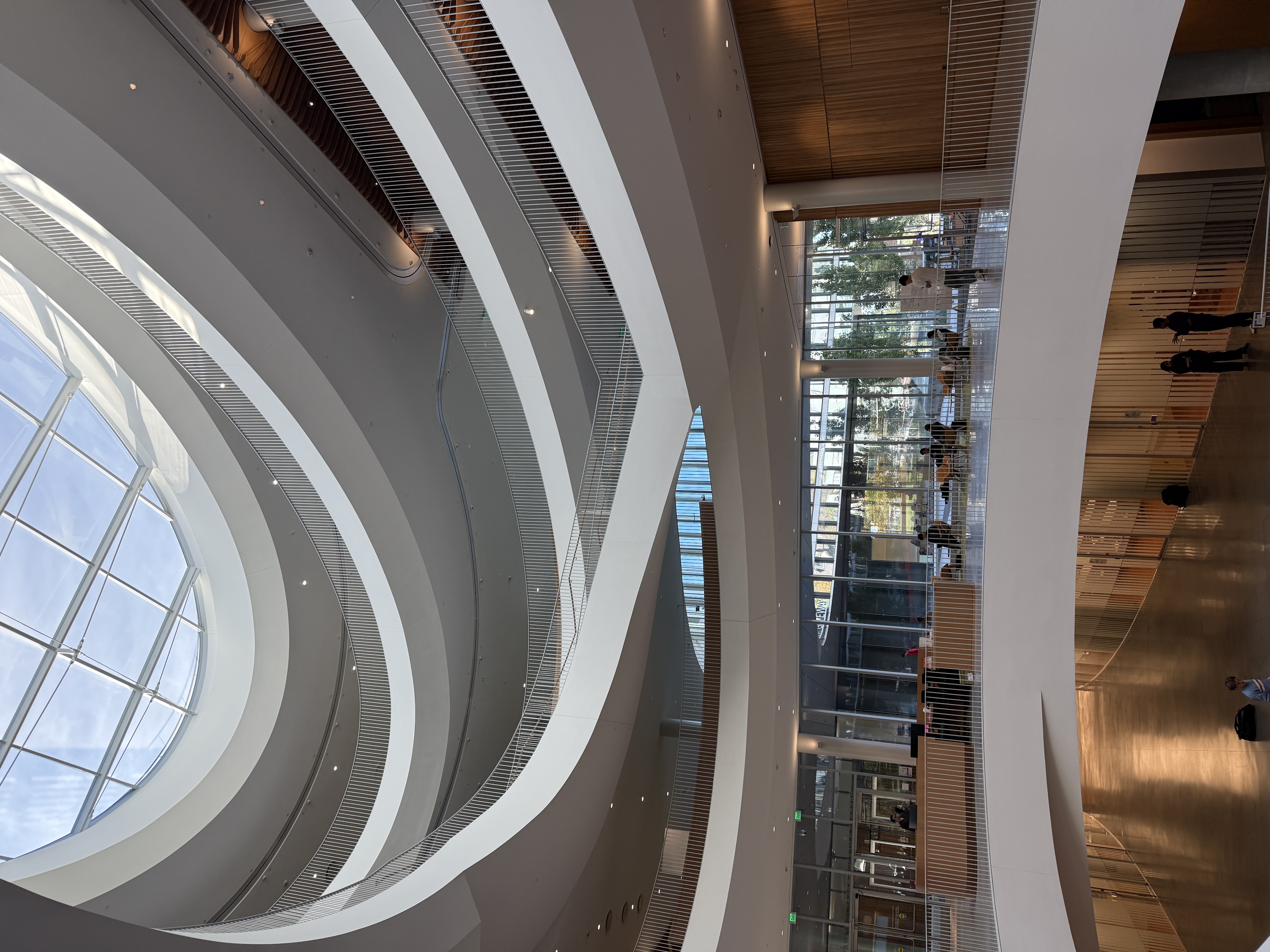
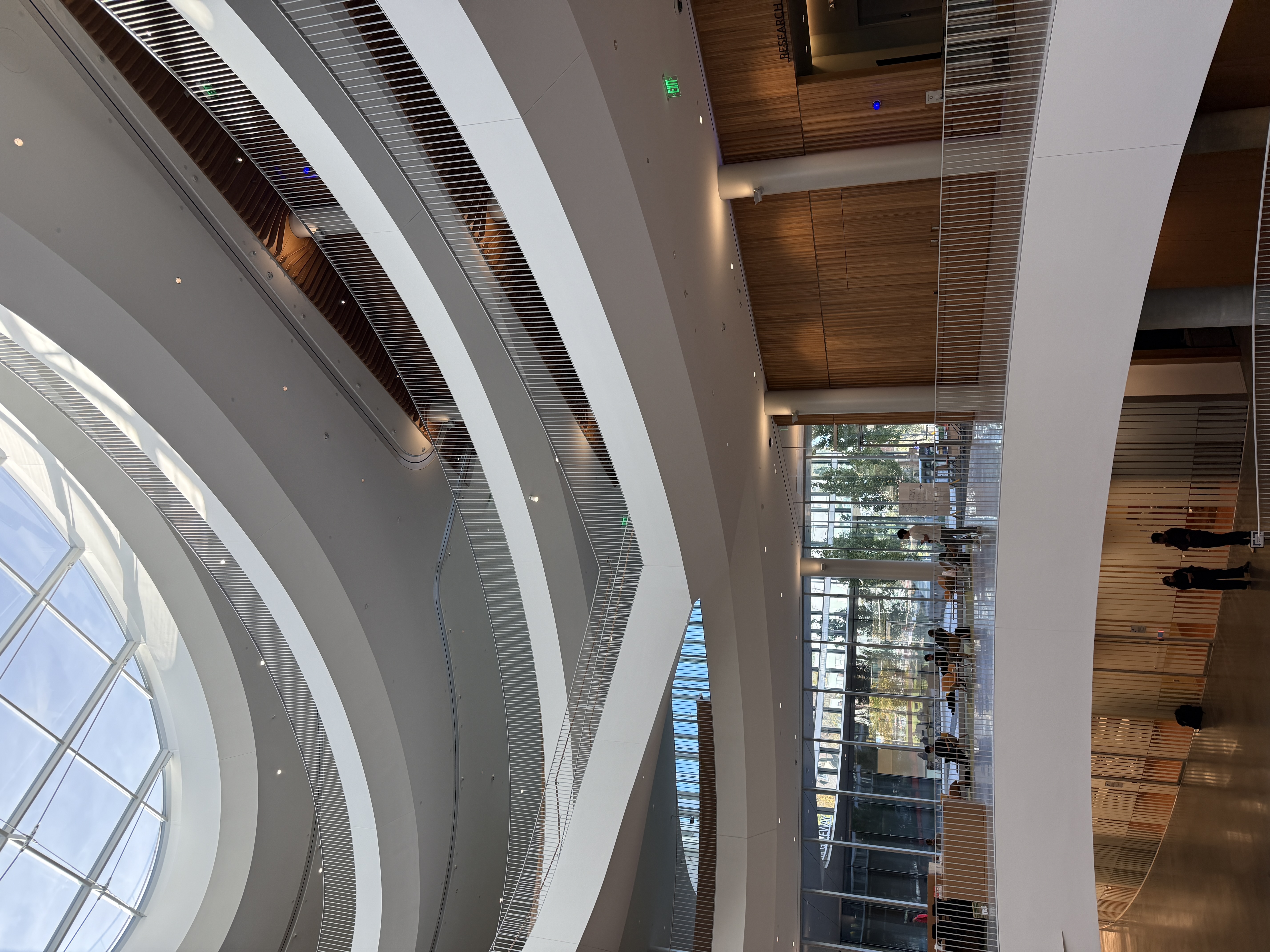
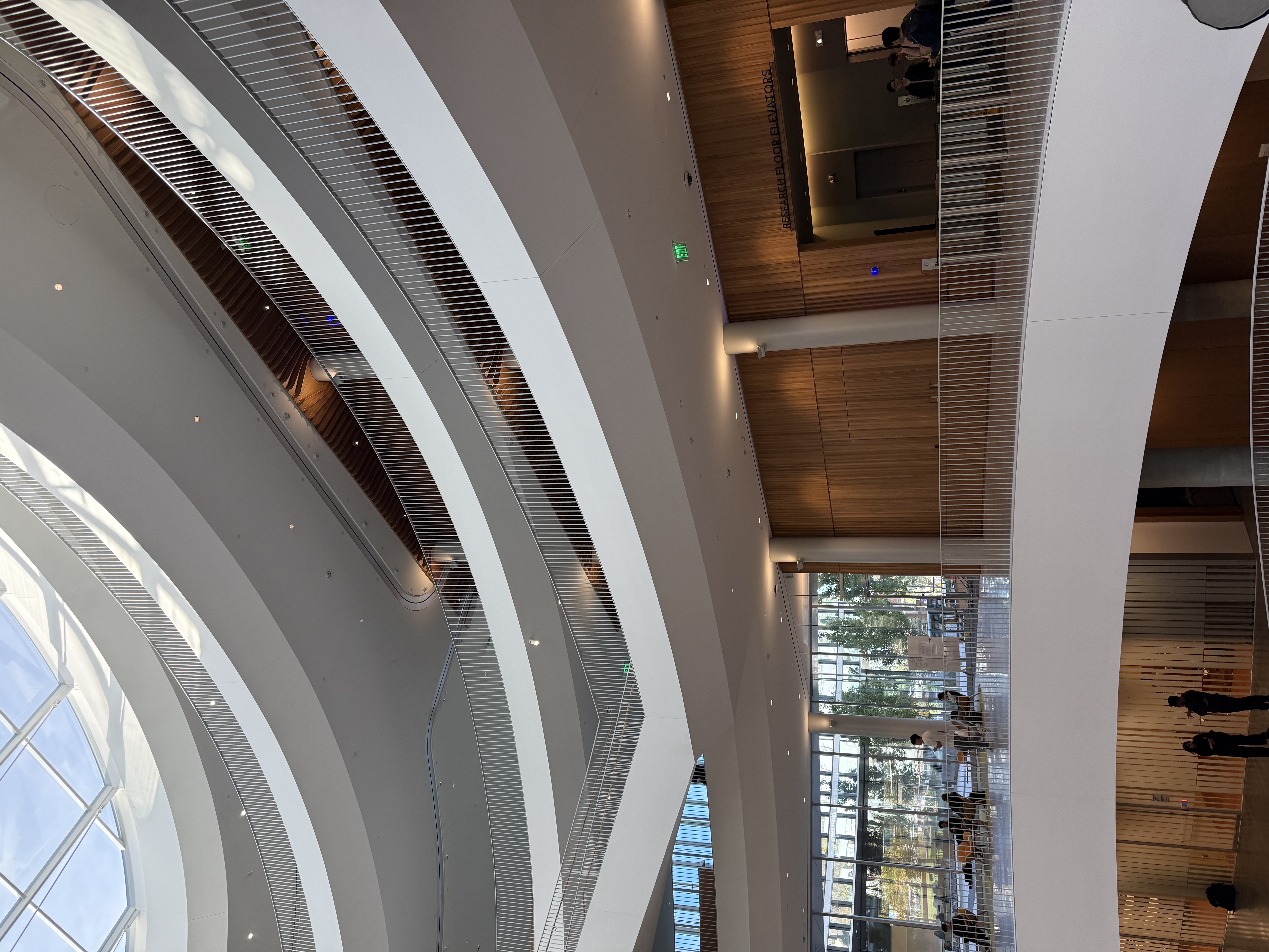
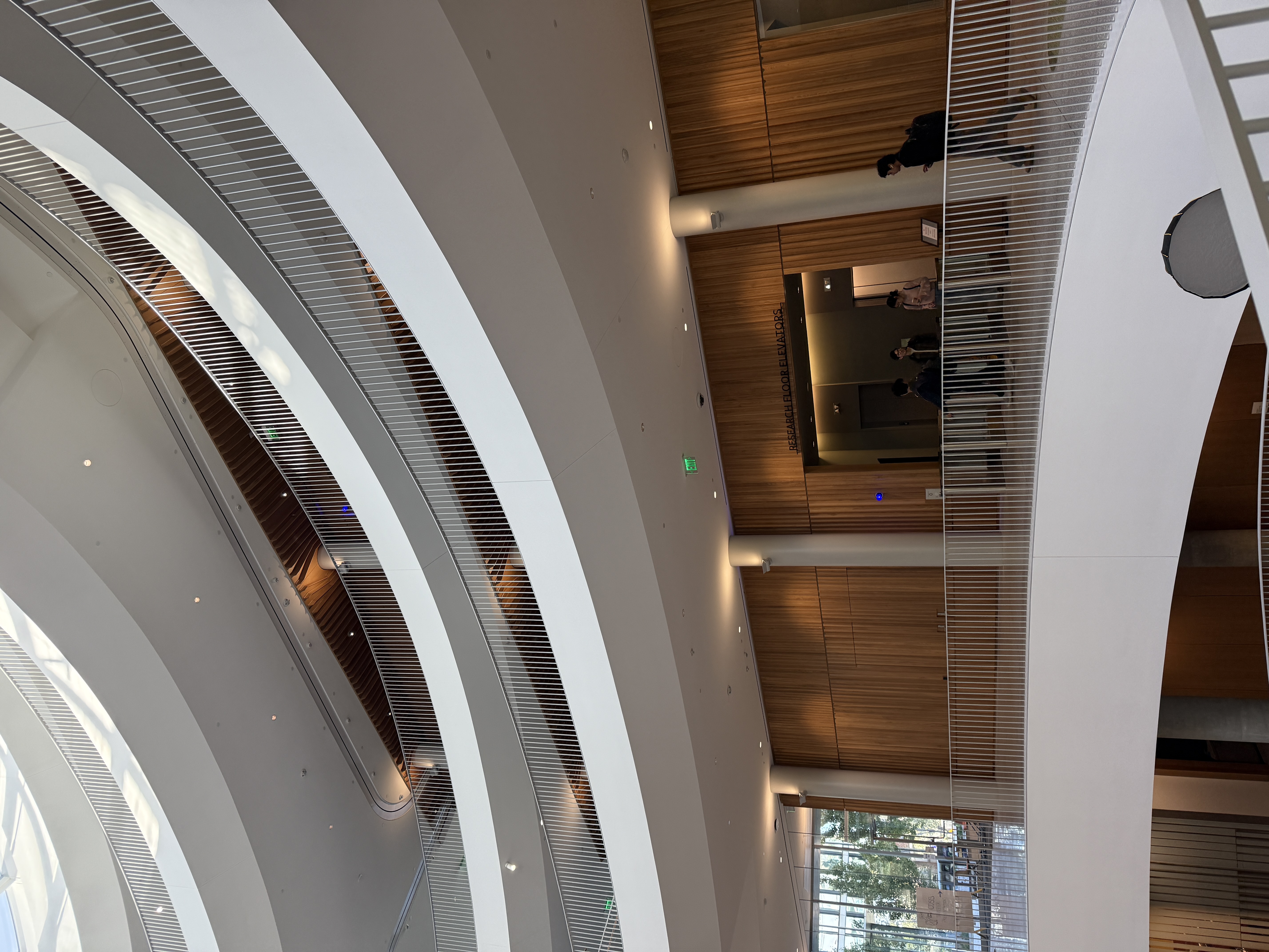
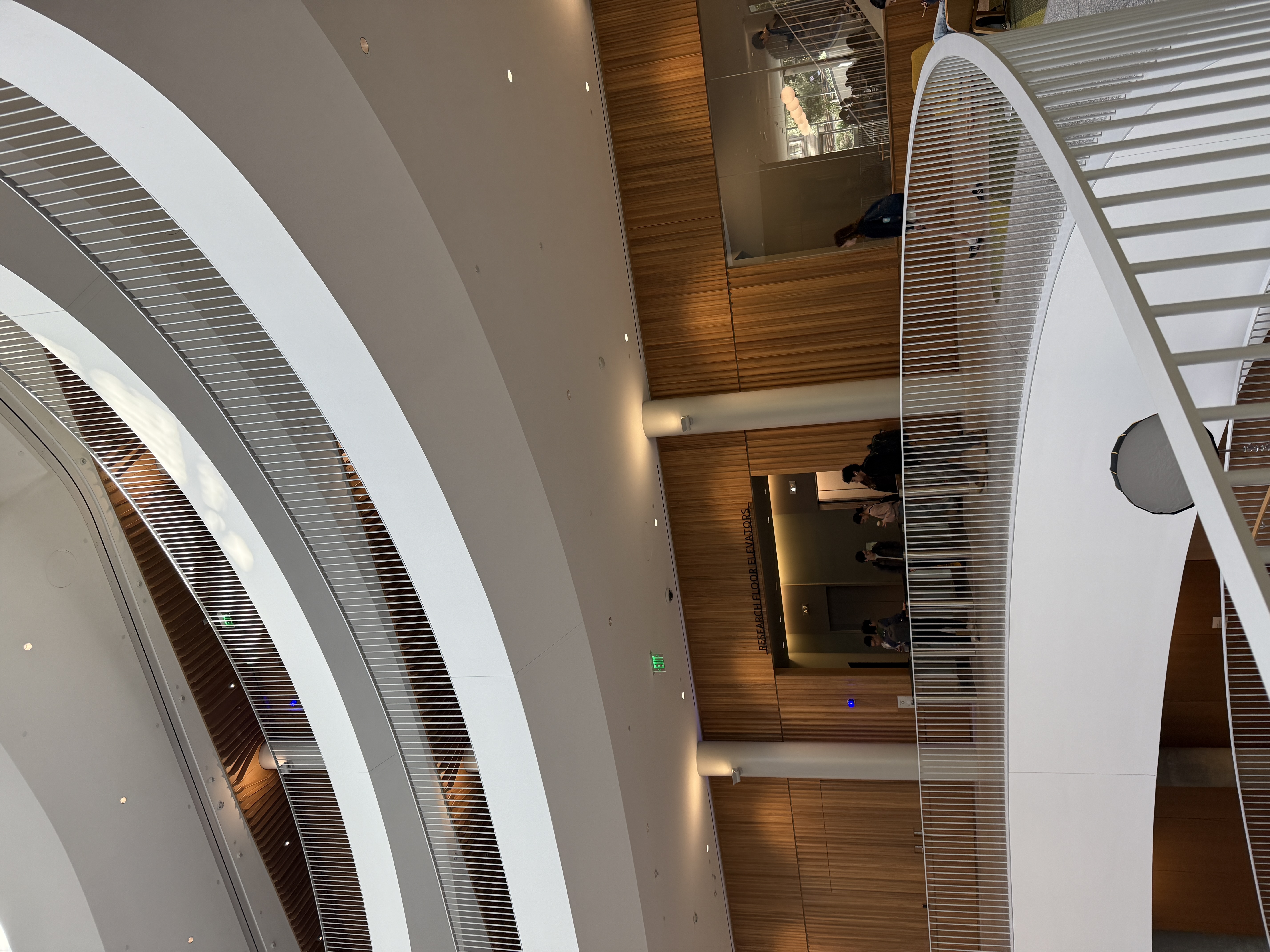
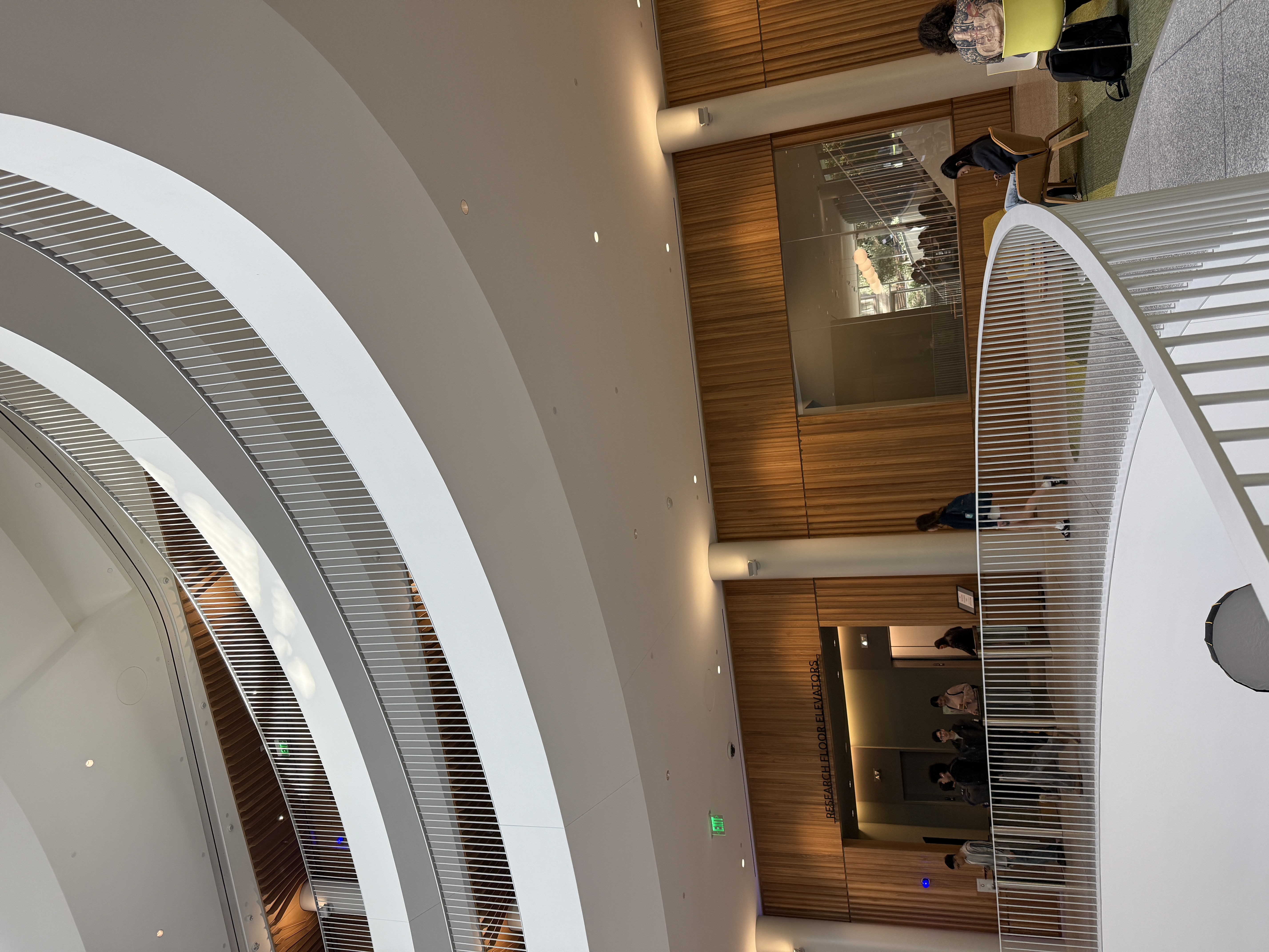
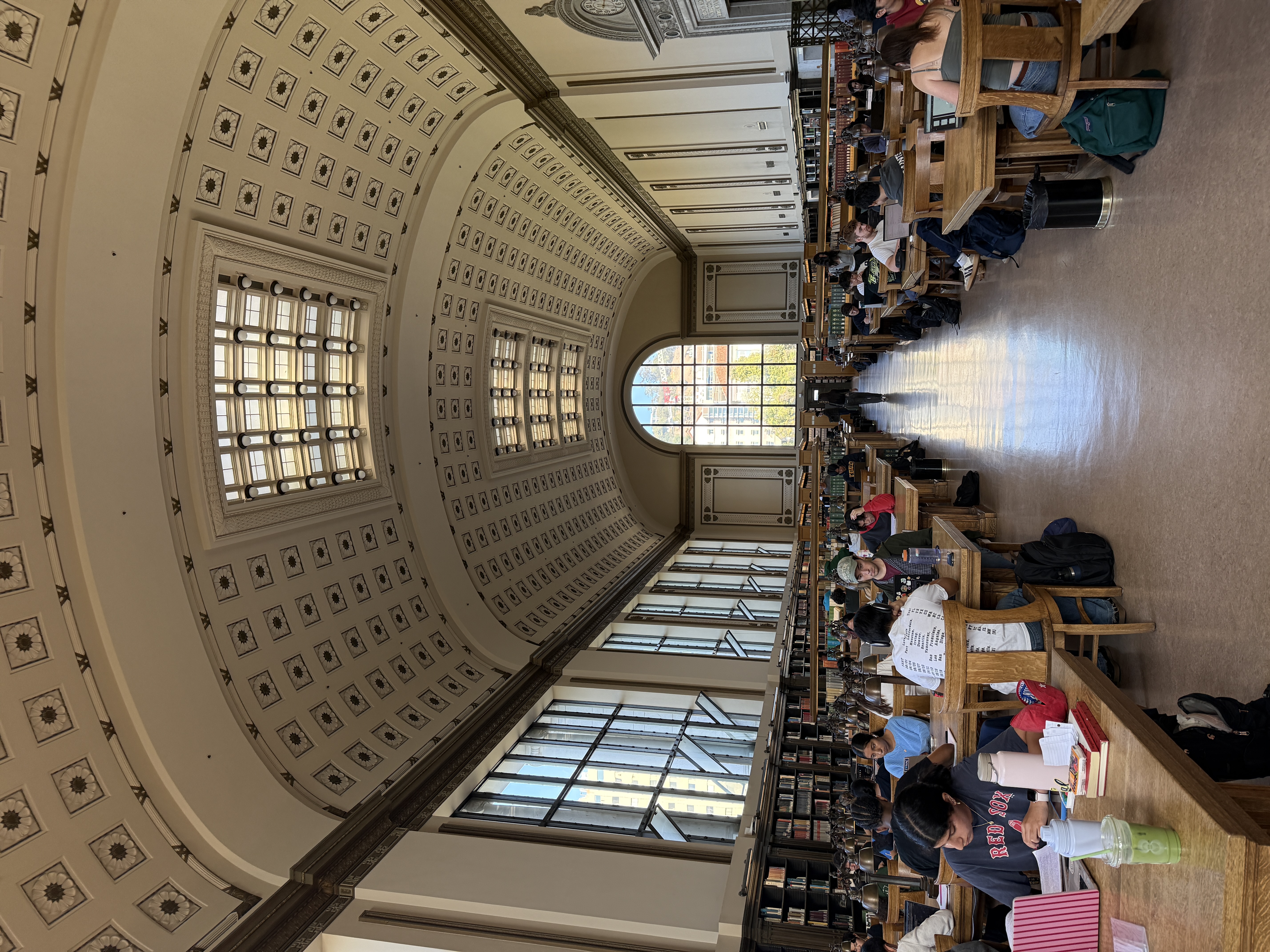
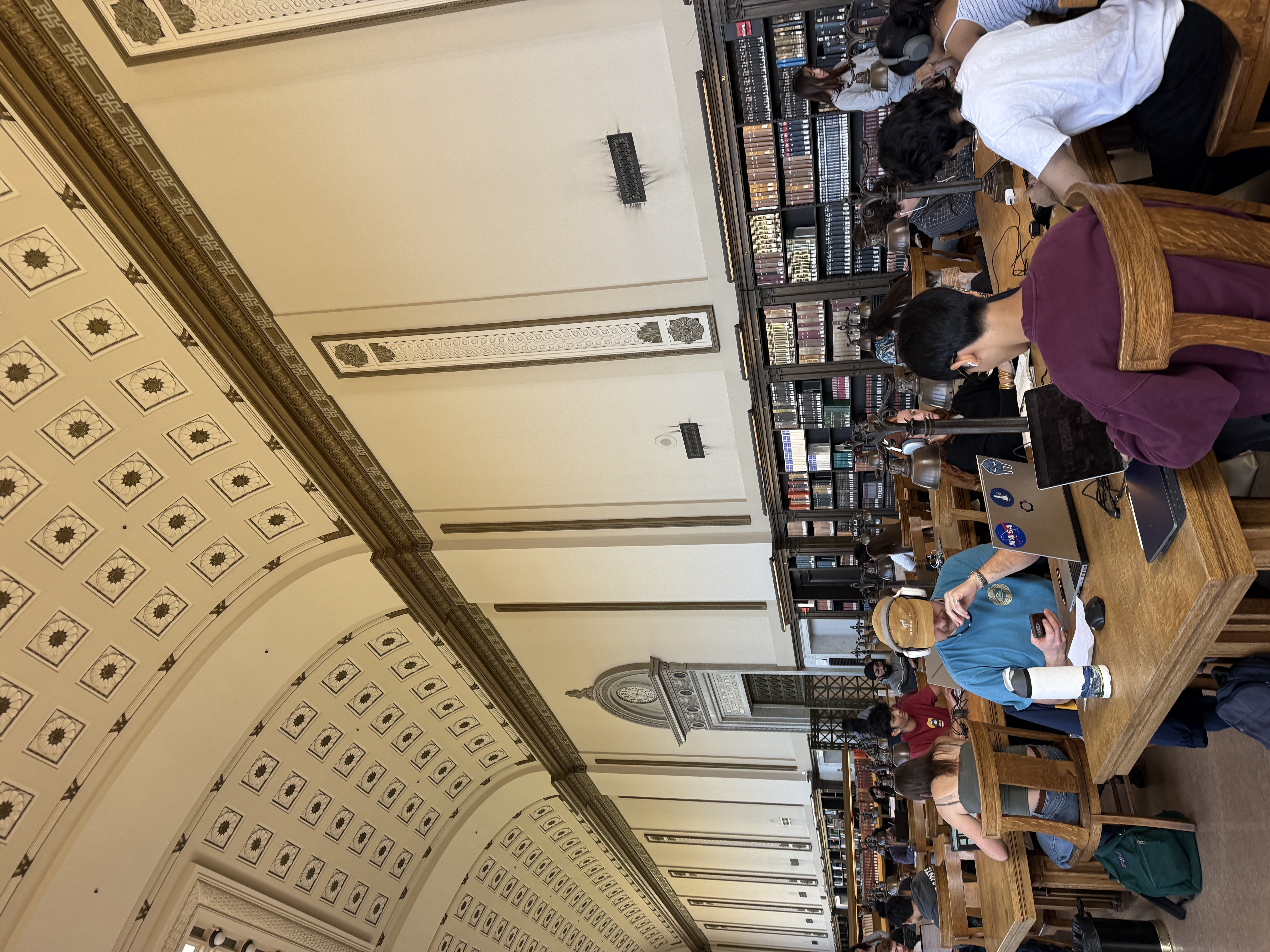
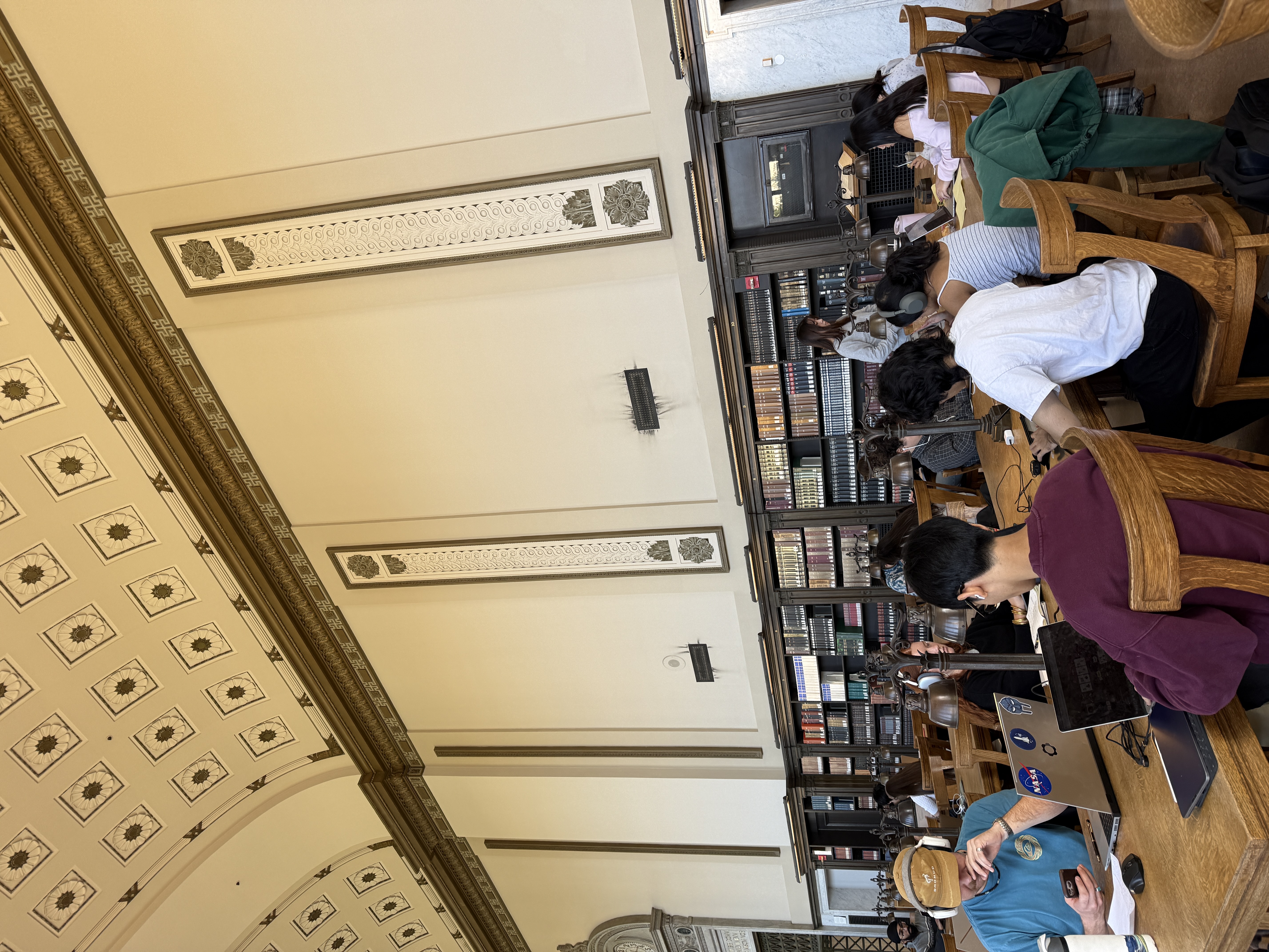
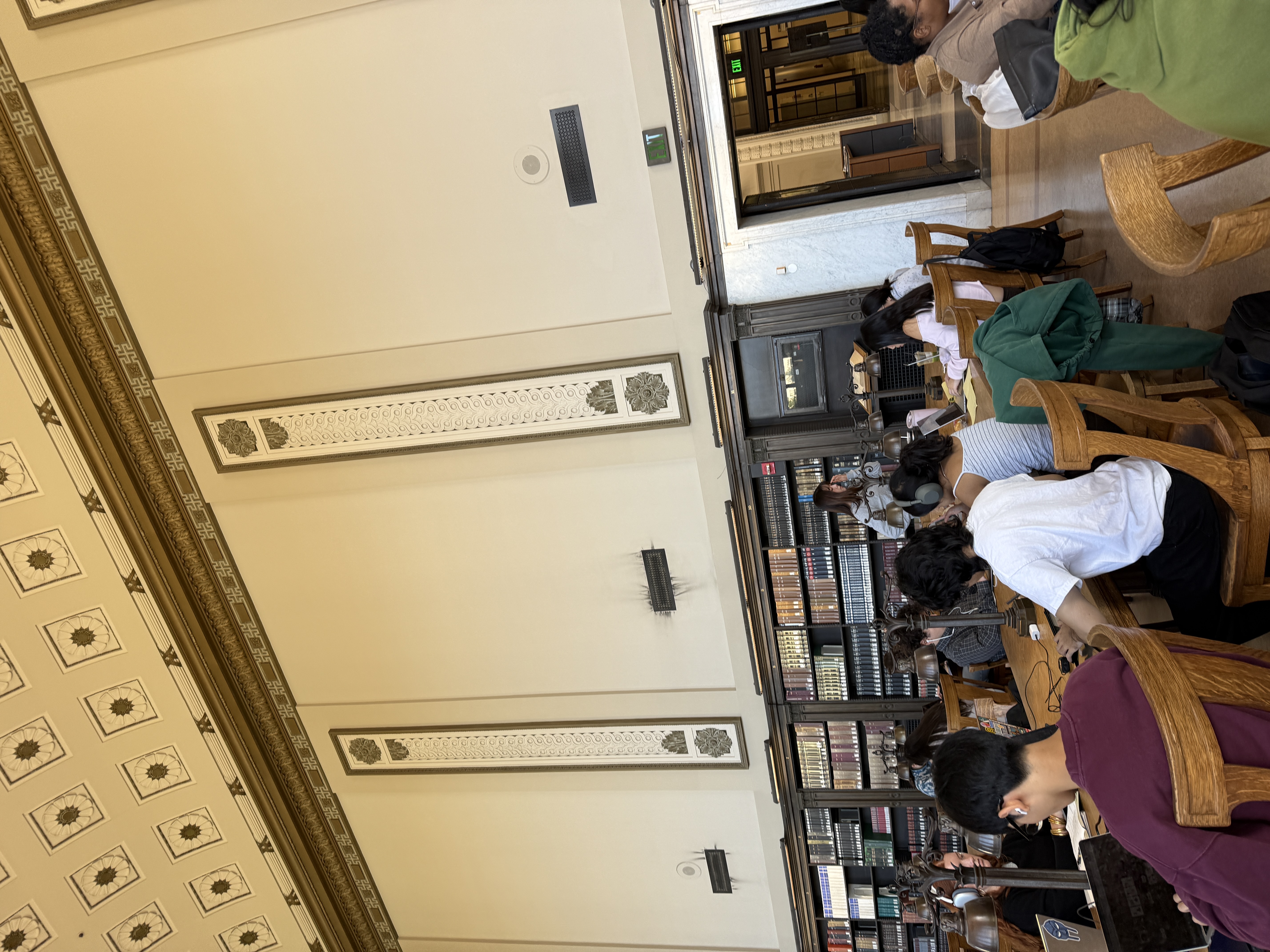
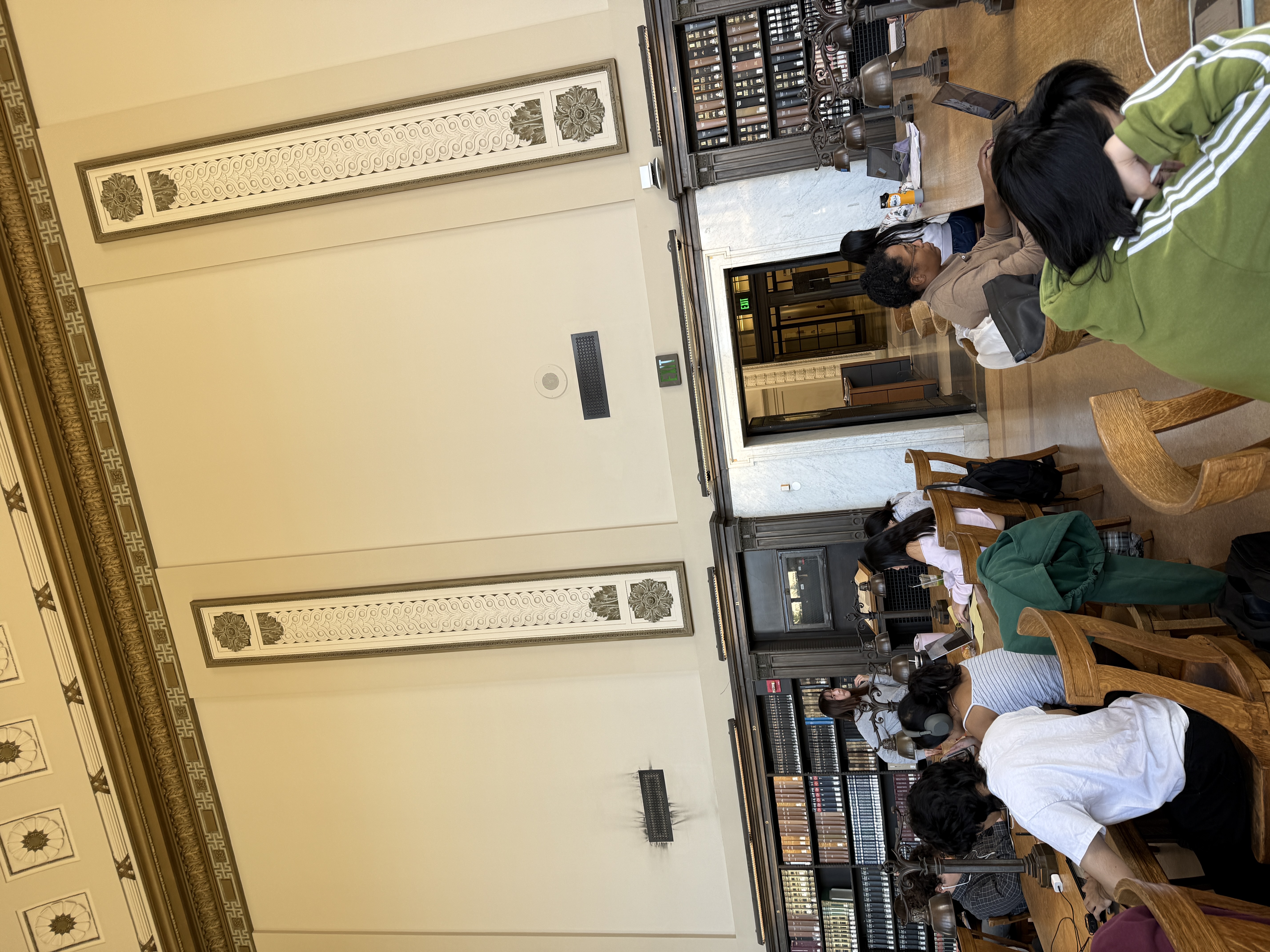
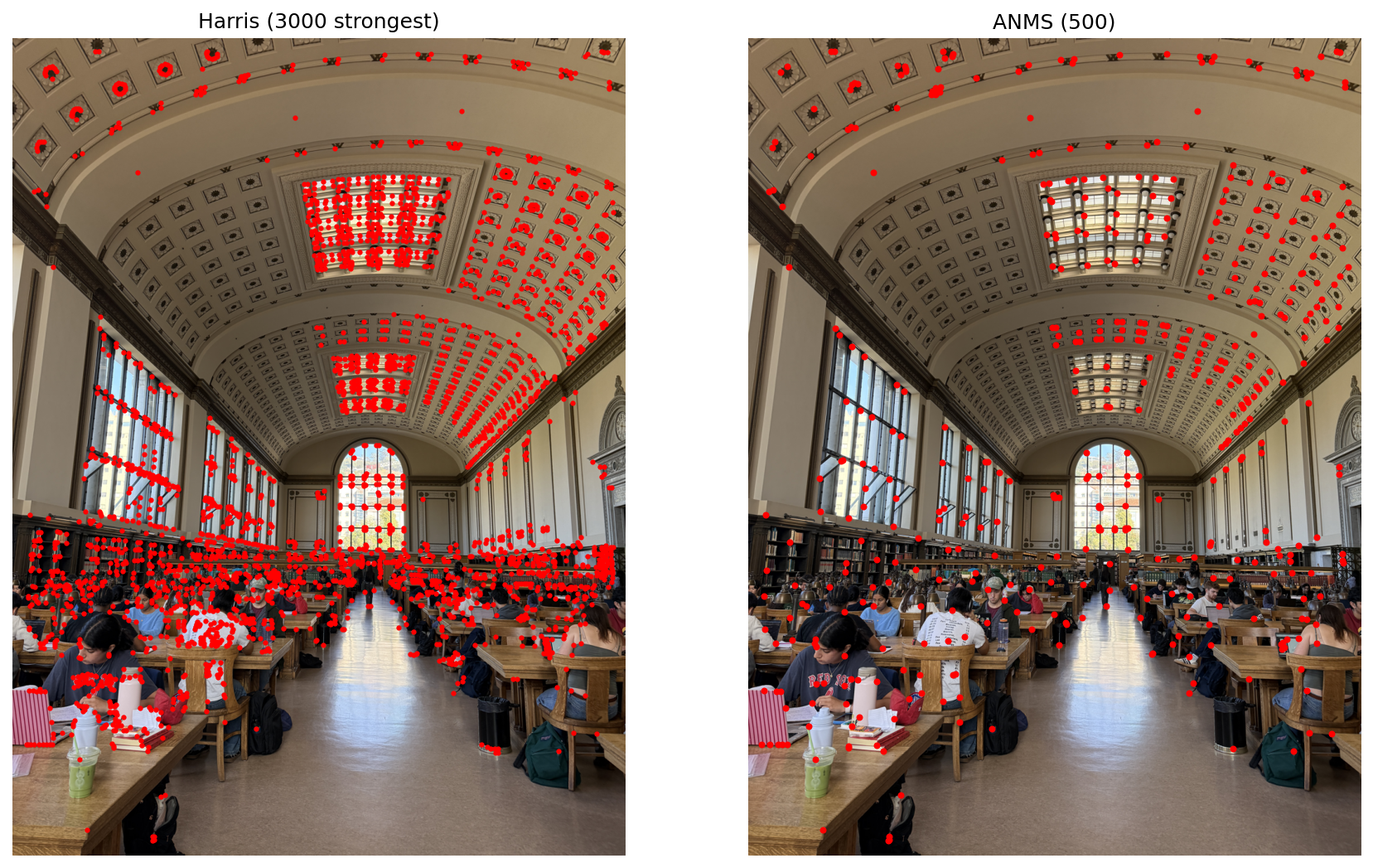
Harris corner detection is a method to detect corners in an image by measuring the change in corner intensity on a grayscale version of the image. High intensity changes happen in areas where the image changes rapidly in 2 directions, whereas low intensity changes are represented by flat areas or straight edges. Corners are defined as the local maxima of the corner strength map, and corners near the border of the image are excluded. In the example to the right, the Harris corner detection kept 3,000 top corners out of 30,000 corners detected, mostly located in high-texture areas such as the ceiling and student study areas.
Adaptive Non-Maximal Suppression (ANMS) is a method for selecting top corner candidates from Harris corner detection by suppressing weak corners within a certain radius of a stronger corner in order to produce an evenly distributed set of corners. For auto-stitching photos, ANMS helps spread corners throughout each image, increasing the chances of finding corresponding corners between images.
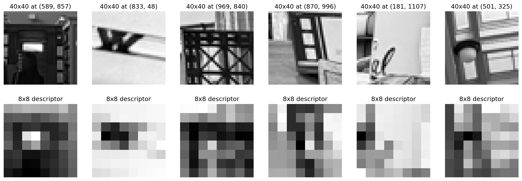
Feature descriptors are used to define the area of interest (around a corner) in an image. For every corner detected and chosen by ANMS, we take a 40x40 window around the corner, turn it into grayscale, blur it, and then average the values in 8x8 patches to get a 64-dimensional descriptor. This descriptor is used to match corners between images. By normalizing the descriptor to ignore brightness and contrast differences, we can more easily match corners with exposure differences. Furthermore, since Harris corners from different photos are detected in different locations, sampling with blurring makes the descriptor less sensitive to small shifts.
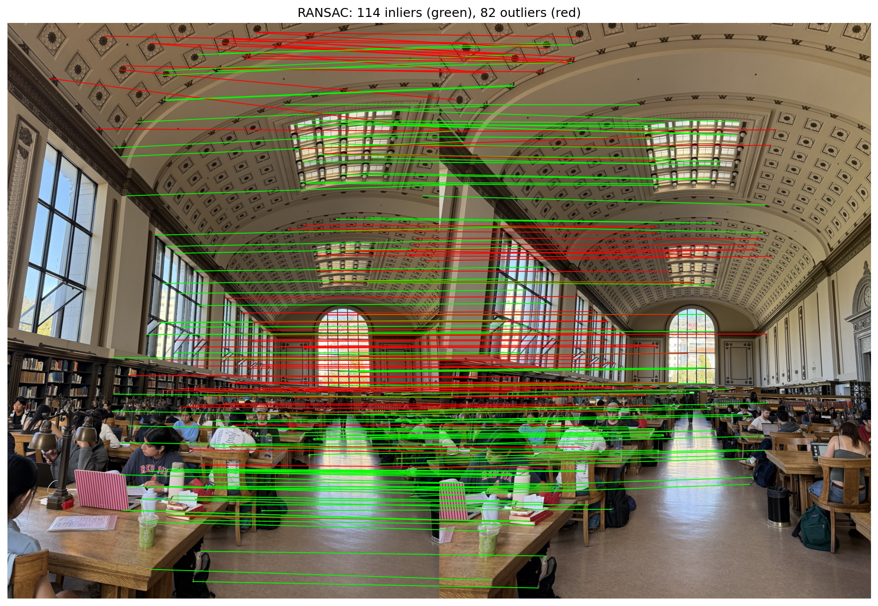
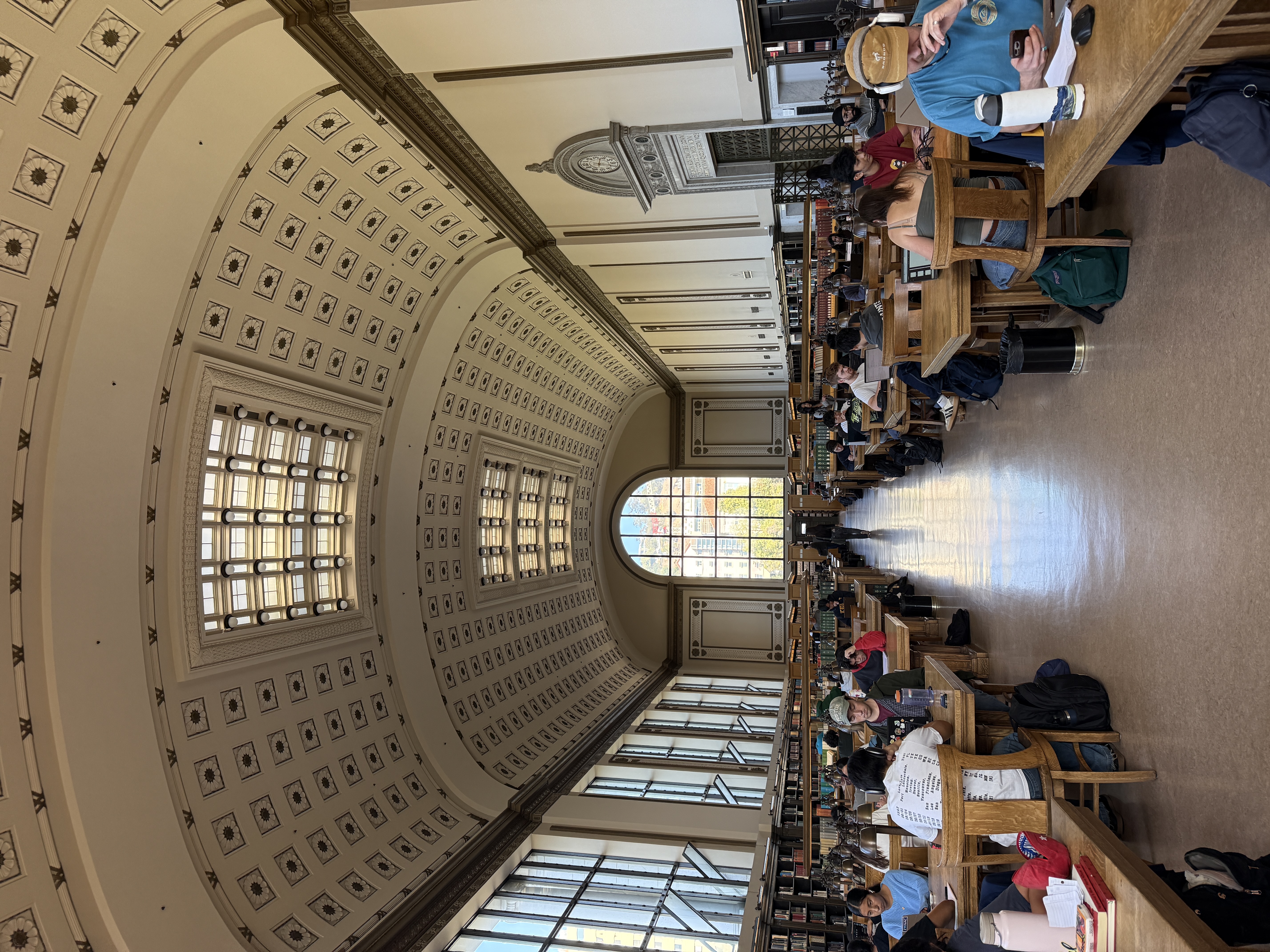
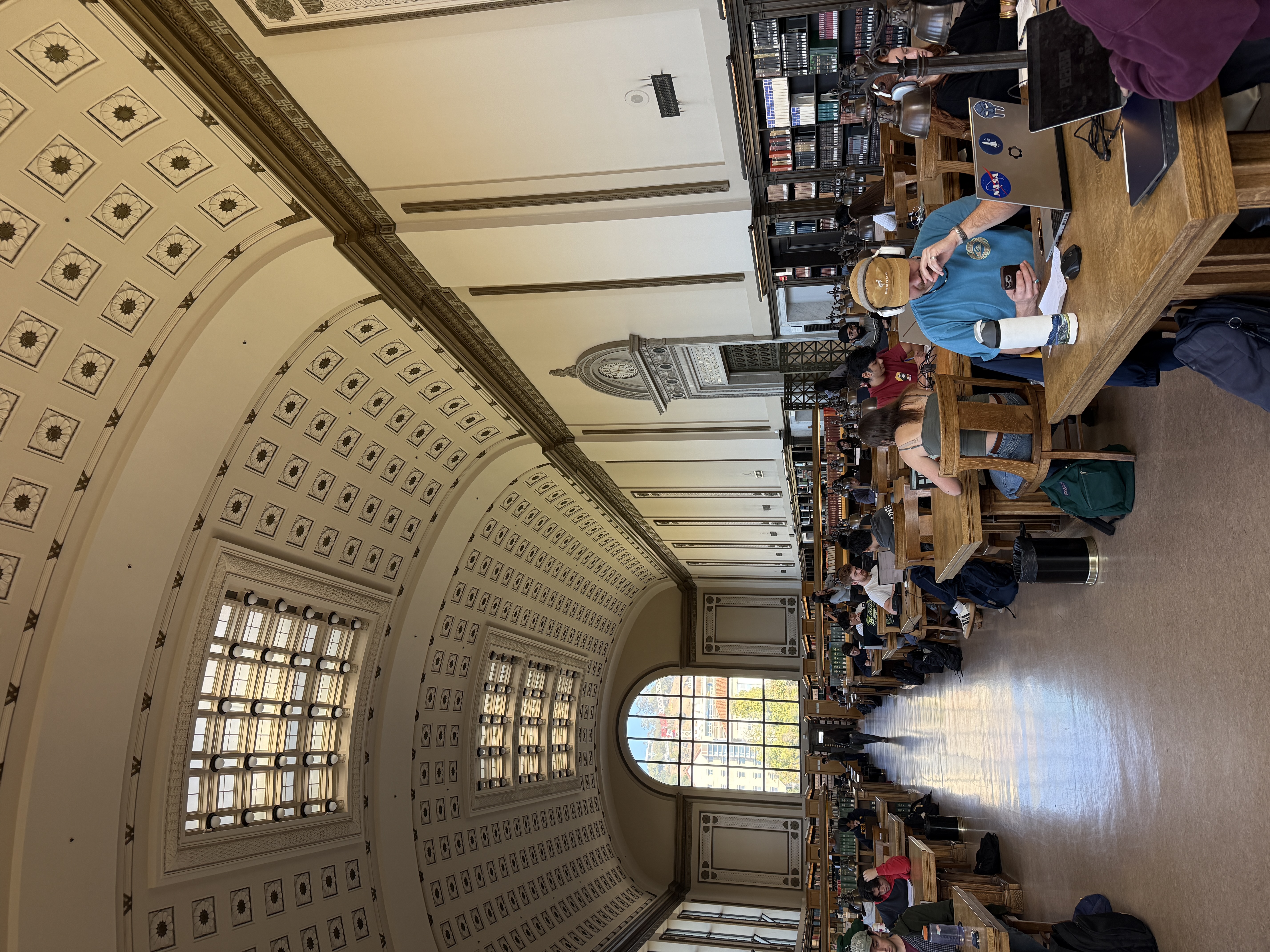
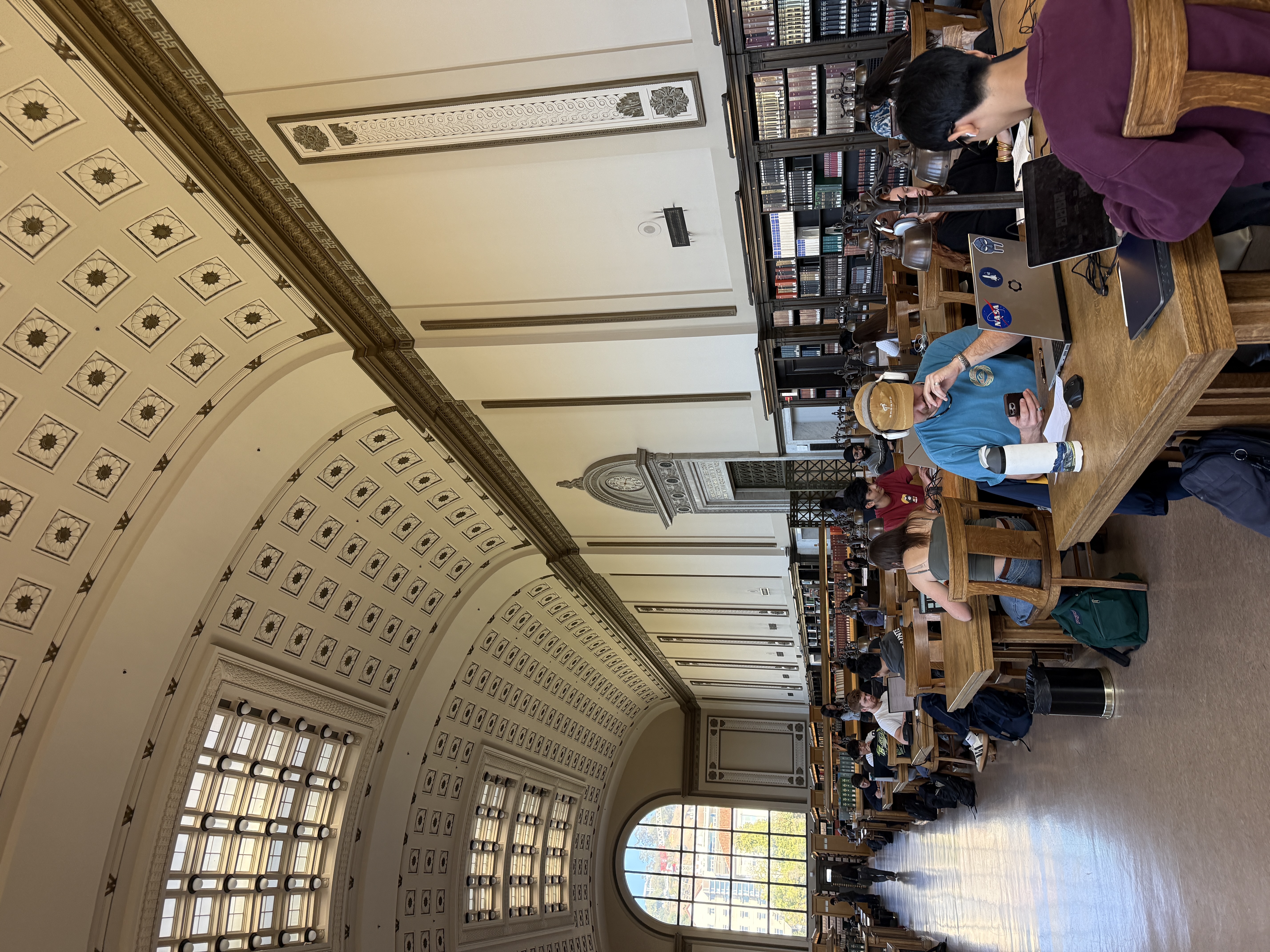
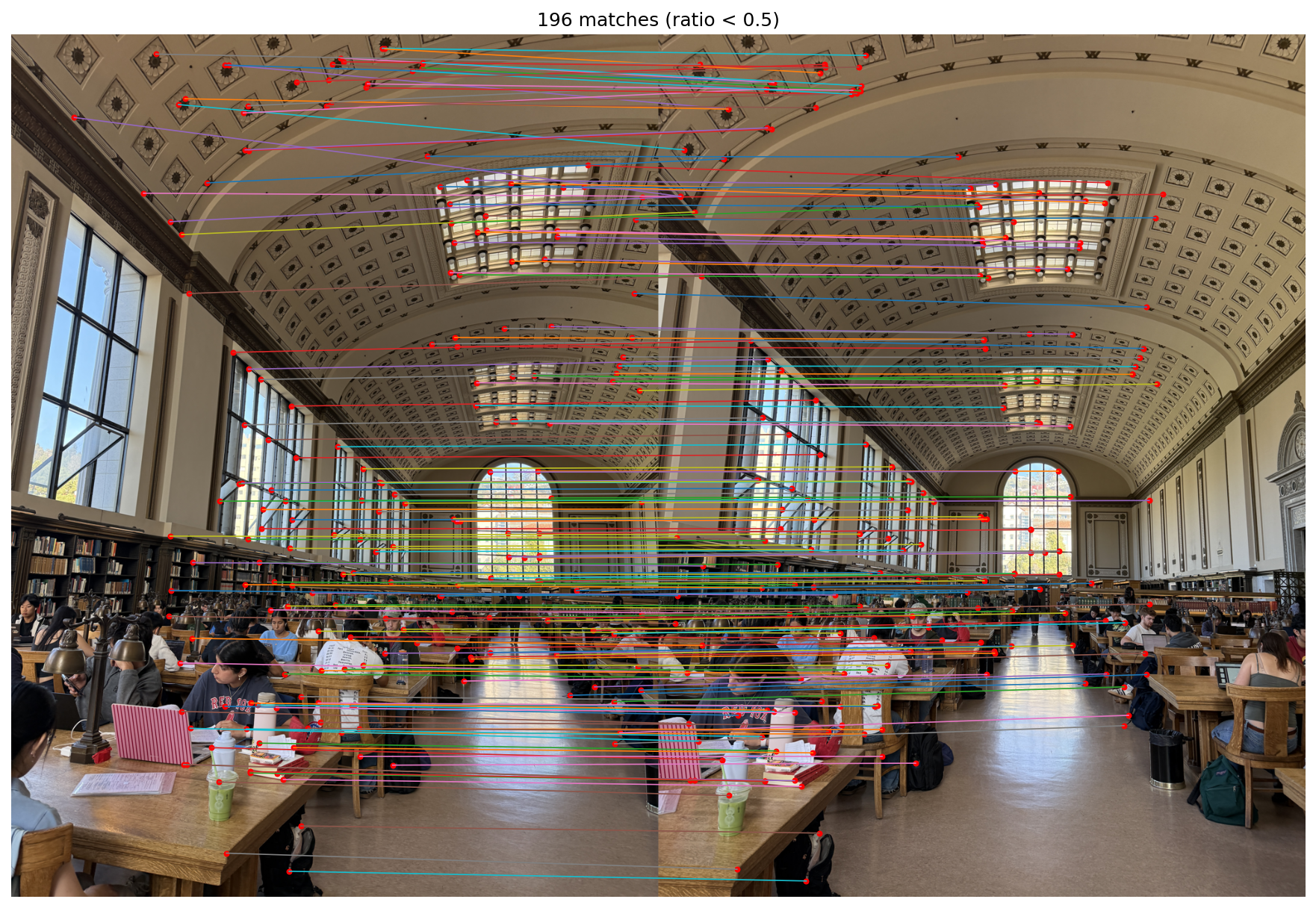
Feature matching is the process of finding corresponding corners between two images by comparing their feature descriptors. By using nearest neighbor matching, we can identify corresponding corners by taking the squared distance between a descriptor in one image and every descriptor in the other image. Since nearest neighbor matching is sensitive to noise, we use Lowe's ratio test where a match is only kept if ratio between the first and second nearest neighbors is less than 0.5, with good matches having smaller ratios. Repetitive patterns like the ceiling tiles have higher ratios, closer to 1. In the example to the right, the ratio test recovered 196 matches between two images of Doe Library, roughly parallel between detailed areas like the ceiling and student study areas. Some incorrect matches resulted from people moving between frames and the repetitive ceiling tiles.
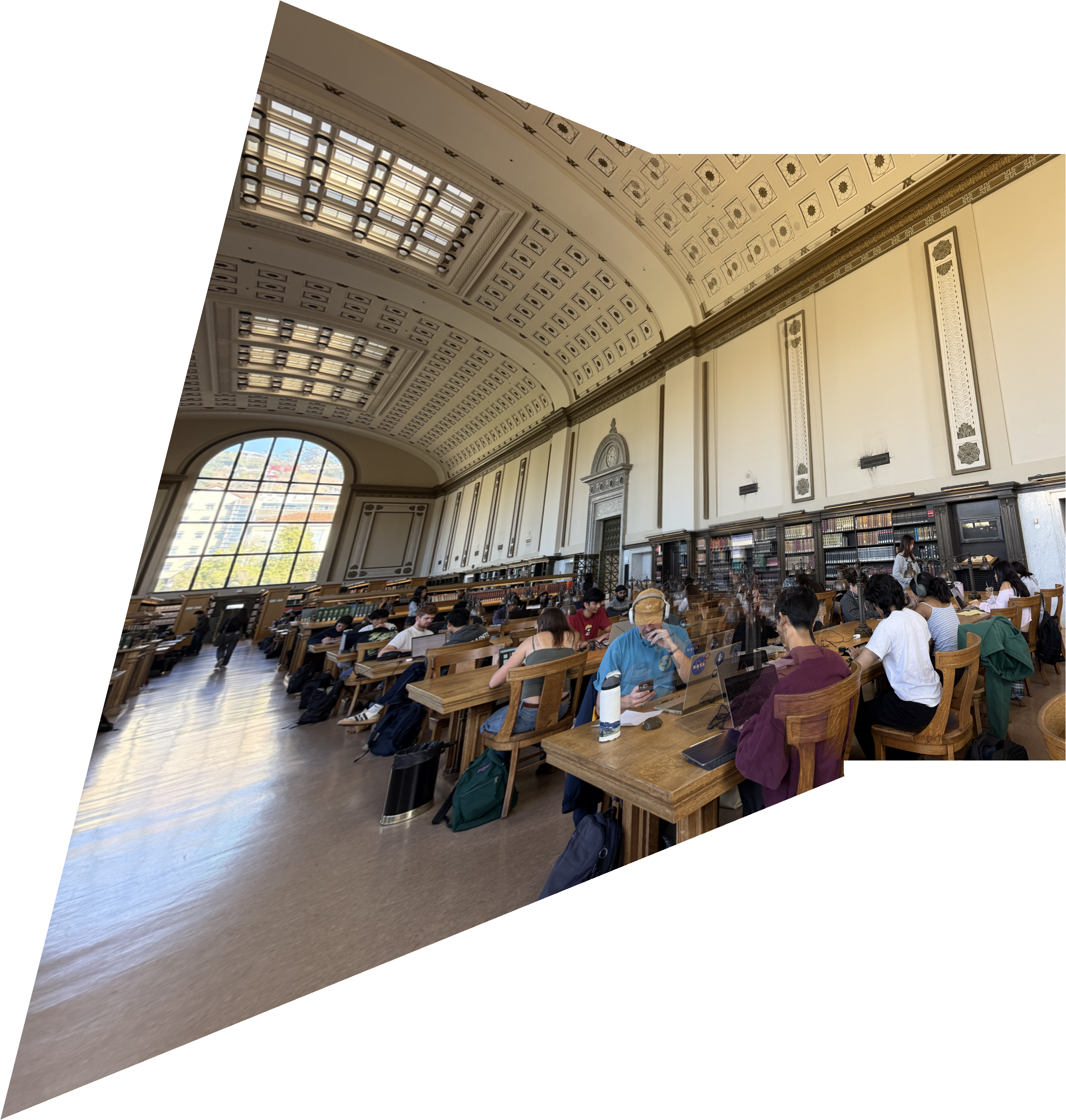
RANSAC is a process for finding the best homography between two images by picking 4 random points and deriving a homography from them. Then, it checks how many matches are inliers, meaning they are within a 2 px threshold of the predicted point. This process is repeated for a set number of iterations (2000), and the homography with the most inliers is kept.
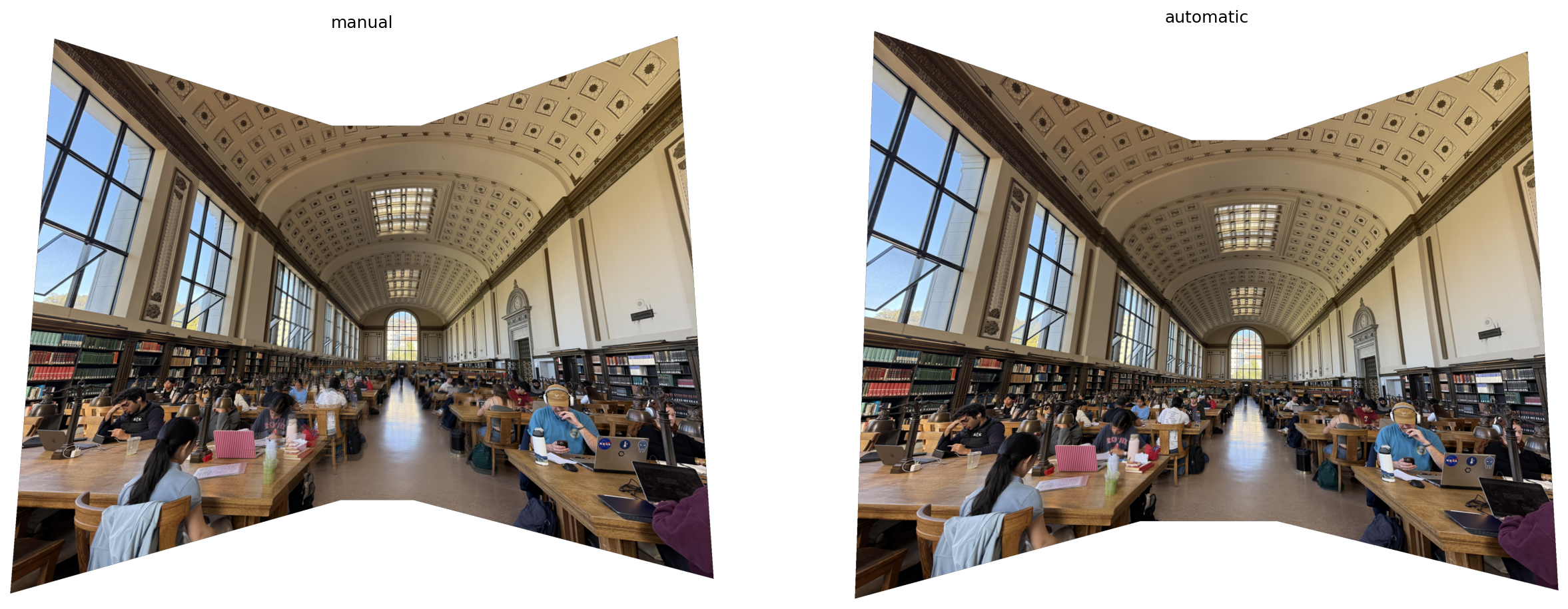
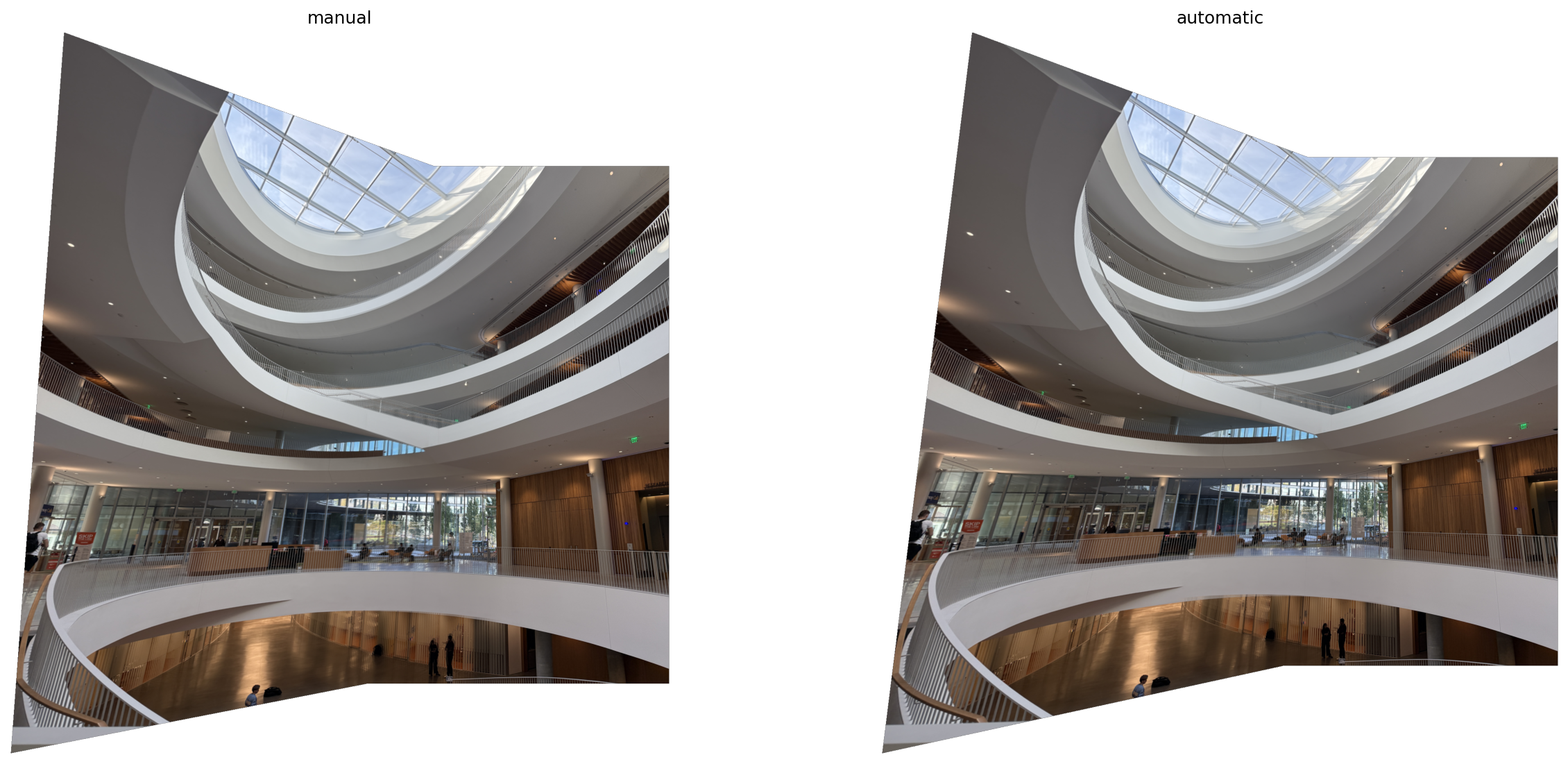
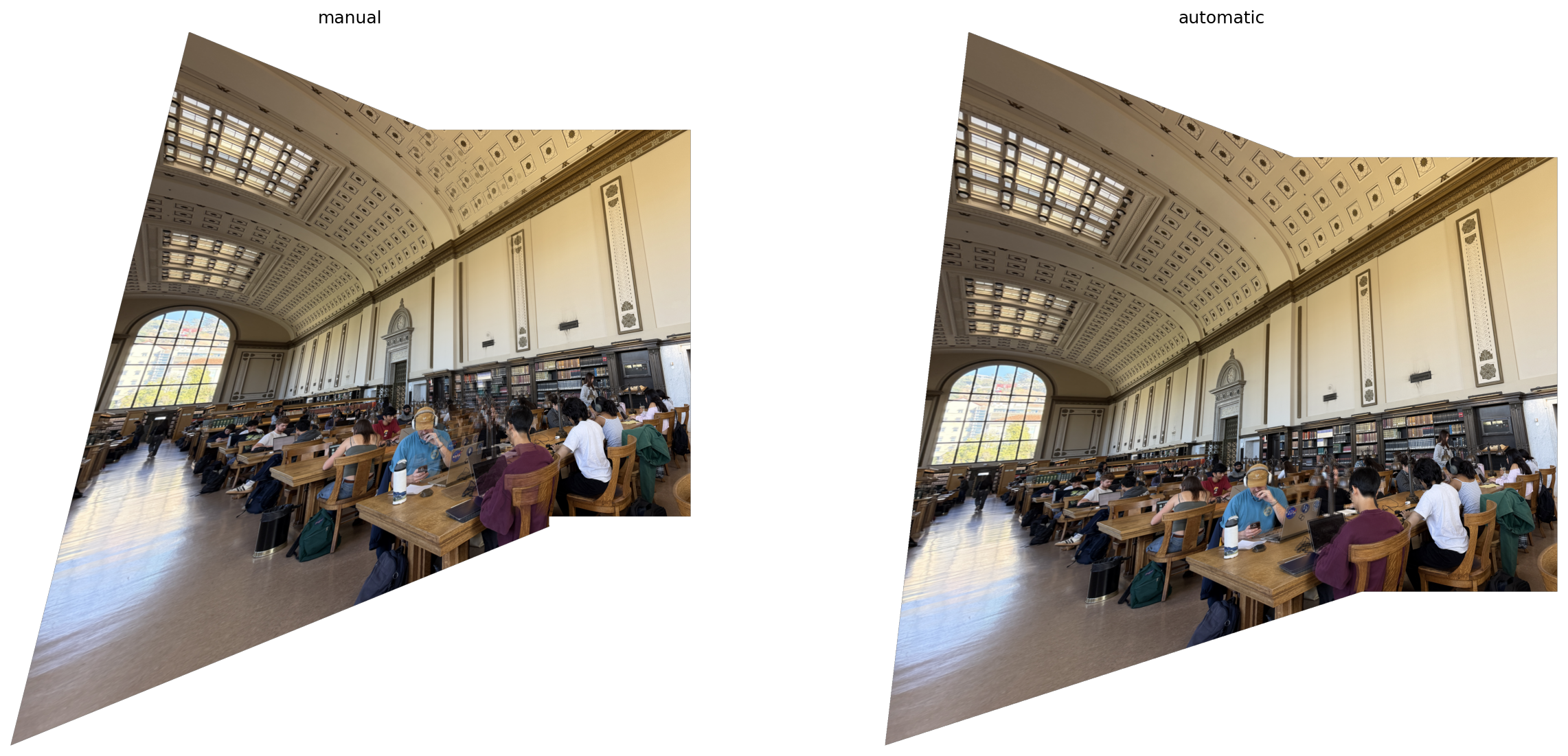
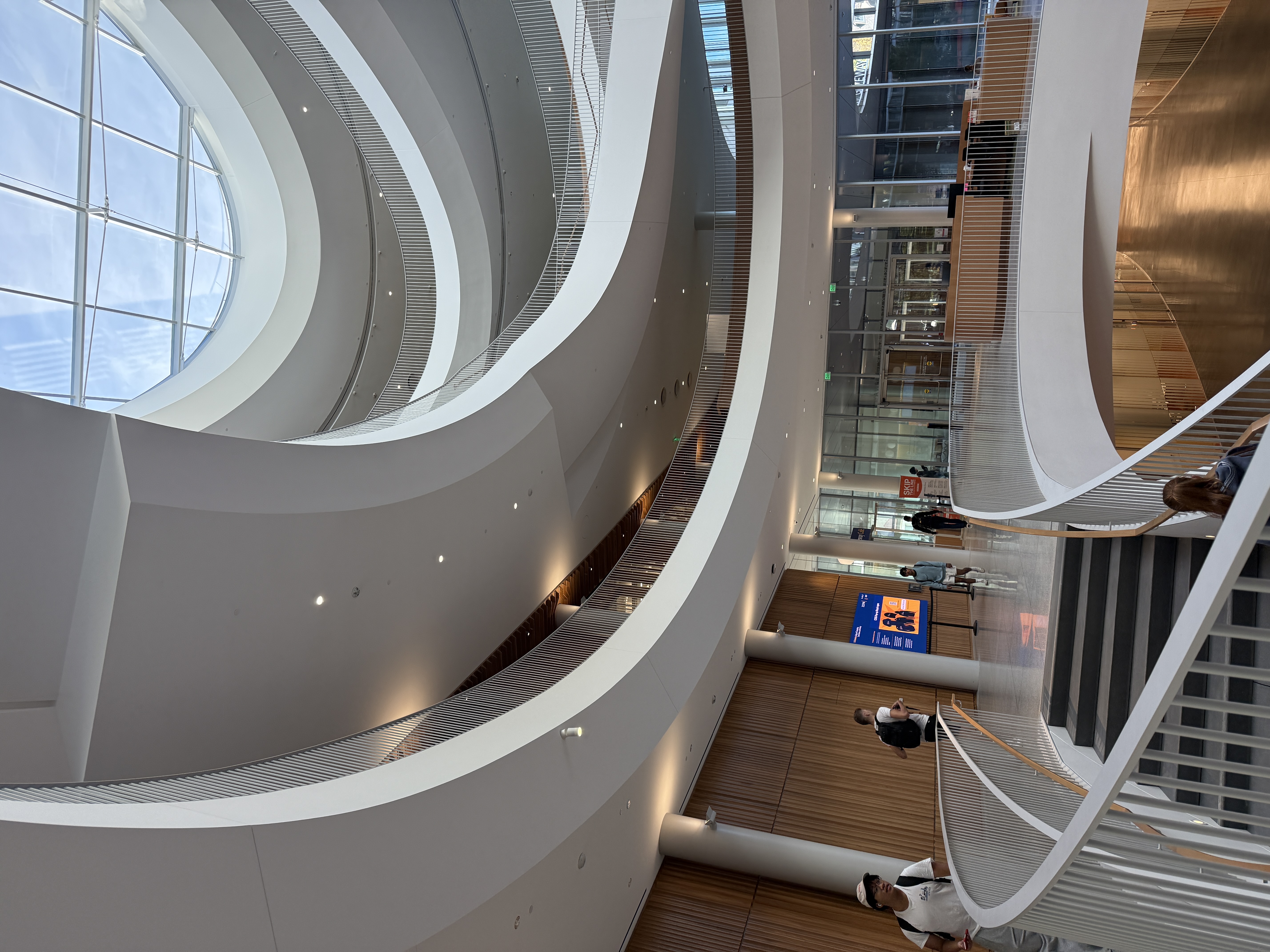
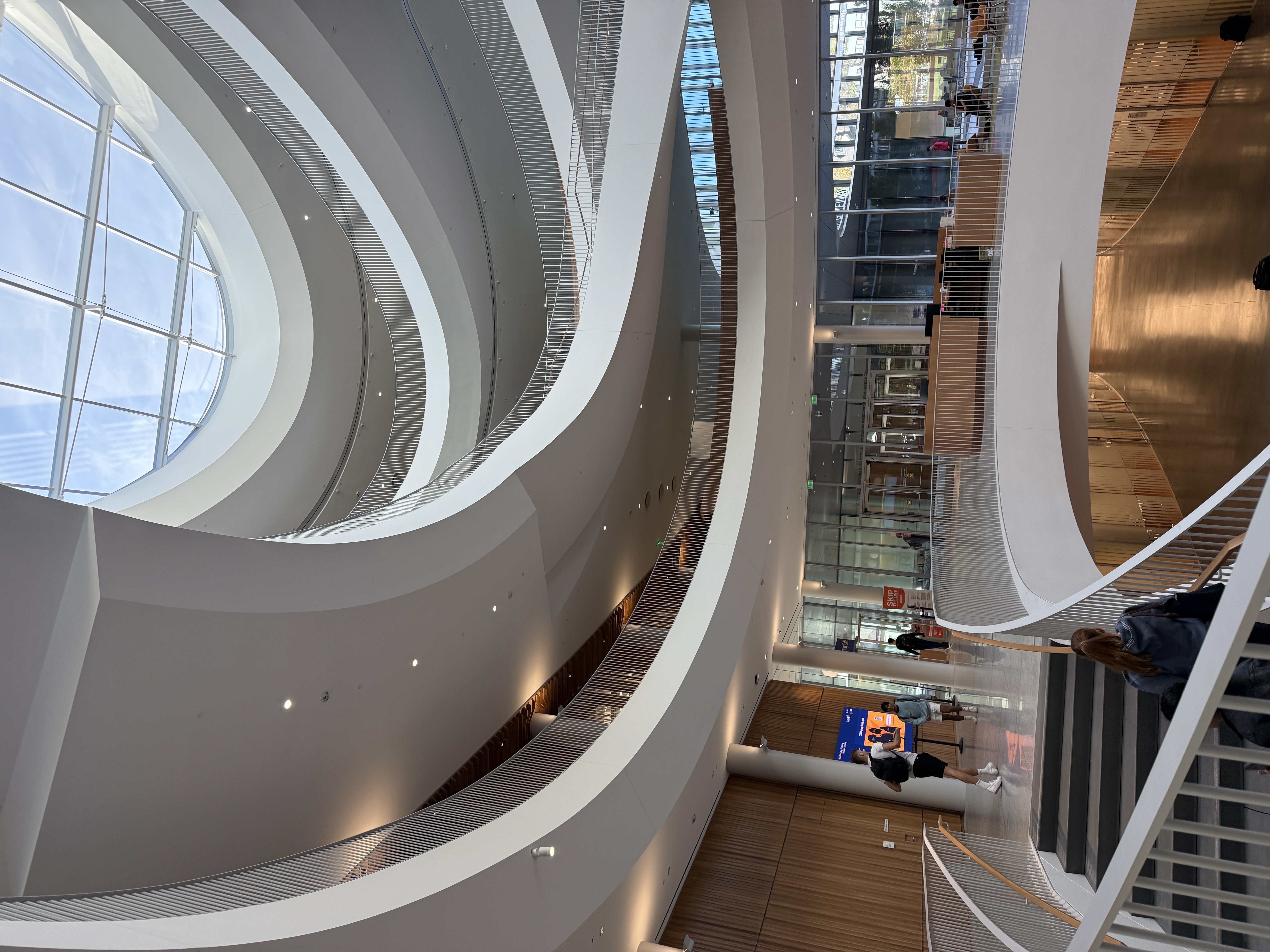
Below are the results of the RANSAC process for multiple images and side by side comparisons of manual vs. automatic stitching.