A convolution creates a new image by applying a kernel (matrix with varying weights and corresponding effects) to the original image. The kernel is applied to each pixel in the original image after getting flipped along the x and y axes, then getting multiplied and summed with the surrounding pixels to produce an output pixel. Examples of kernel effects include a matrix with equal weights (blurring effect) and a finite difference kernel (which uses subtraction to detect edges).
def padding(im, kh, kw):
    top = kh // 2
    bottom = (kh - 1) // 2
    left = kw // 2
    right = (kw - 1) // 2
    H, W = im.shape
    padded = np.zeros((H + top + bottom, W + left + right), dtype=np.float64)
    padded[top:top + H, left:left + W] = im
return paddeddef convolution_four(im, kernel):
kh, kw = kernel.shape
k = kernel[::-1, ::-1] # flip the kernel
padded = padding(im, kh, kw)
H, W = im.shape
out = np.zeros((H, W), dtype=np.float64)
for i in range(H):
for j in range(W):
total = 0.0
for m in range(kh):
for n in range(kw):
total += padded[i + m, j + n] * k[m, n]
out[i, j] = total
return outdef convolution_two(im, kernel):
kh, kw = kernel.shape
k = kernel[::-1, ::-1]
padded = padding(im, kh, kw)
H, W = im.shape
out = np.zeros((H, W), dtype=np.float64)
for i in range(H):
for j in range(W):
out[i, j] = np.sum(padded[i:i + kh, j:j + kw] * k)
return outscipy_result = scipy.signal.convolve2d(im, k, mode="same", boundary="fill", fillvalue=0)box = np.ones((9, 9)) / 81.0
Dx = np.array([[1, -1]], dtype=np.float64)
Dy = np.array([[1], [-1]], dtype=np.float64)| Implementation | Runtime (9x9 box) | Relative to SciPy |
|---|---|---|
| Four loops | 5.397 s | ~151x slower |
| Two loops + NumPy | 0.716 s | ~20x slower |
scipy.signal.convolve2d |
0.036 s | 1x (baseline) |
| Kernel | Four loops vs SciPy | Two loops vs SciPy |
|---|---|---|
| 9x9 box | 8.88e-16 | 8.88e-16 |
| Dx = [1, -1] | 0.0 | 0.0 |
| Dy = [1, -1]T | 0.0 | 0.0 |
All implementations, convolution_four, convolution_two, and scipy.signal.convolve2d, use the same boundary rule of zero padding. With convolutions, every kernel weight is multiplied with a pixel from the original image. However, at the border, the kernel will stick out, and thus, missing pixels are treated as and padded with zeros so that the output and input images are the same sizes. In the presented implementations, convolution_four and convolution_two use np.zeros to create the padding, whereas SciPy uses scipy.signal.convolve2d(im, k, mode="same", boundary="fill", fillvalue=0)
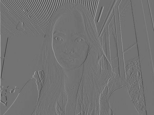
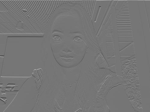
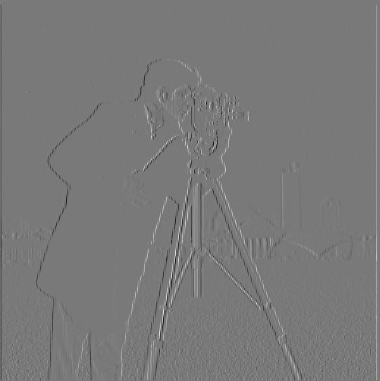
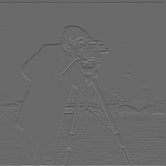
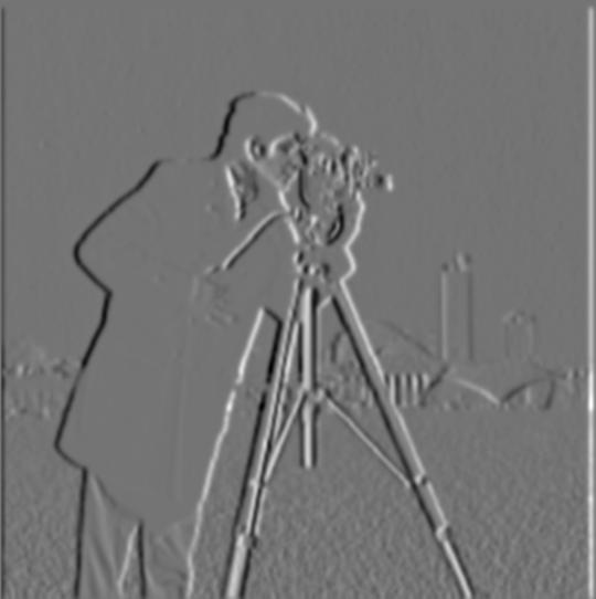
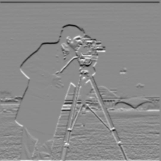
To find edges in the cameraman image, I convolved it with finite difference operators Dx using scipy.signal.convolve2d. This creates output pixels which represent the difference between a pixel in the original image and its neighbor. Thus, if the two values are the same, the difference is zero in a flat area, and the difference is larger when there is a greater change in value, representing an edge. Since Dx measures from left to right, it creates vertical edges; similarly, since Dy measures from top to bottom, it creates horizontal edges. boundary="symm" was used to handle borders instead of zero padding since zero padding would create a false edge at the border.
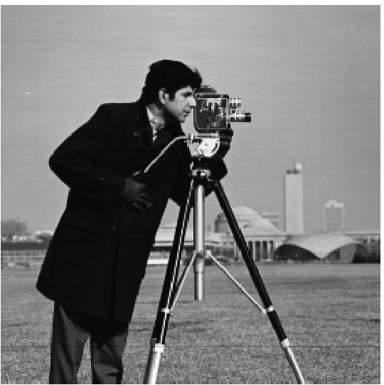
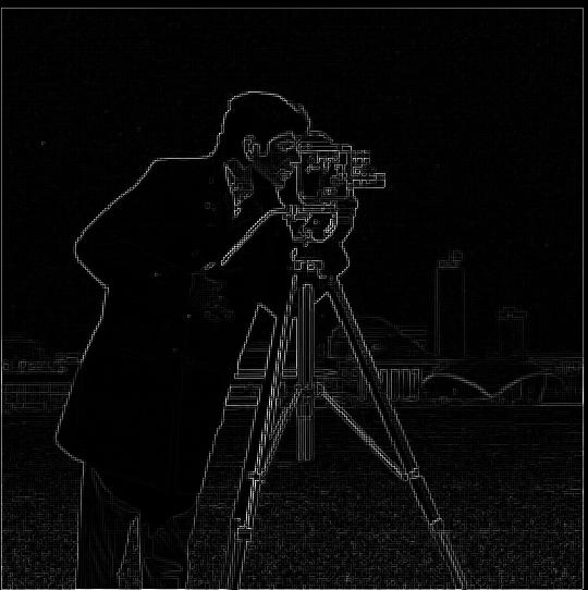
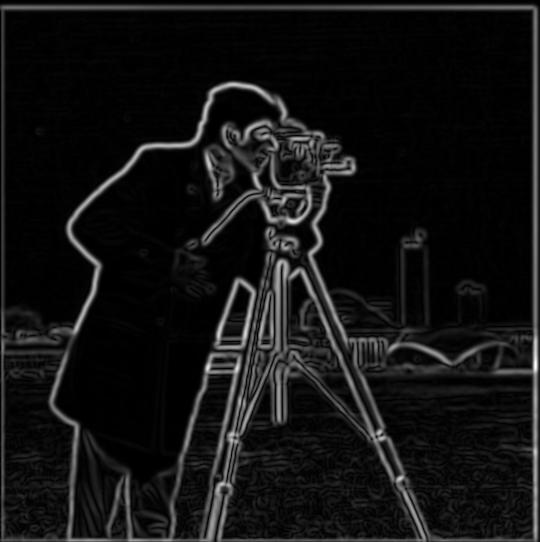
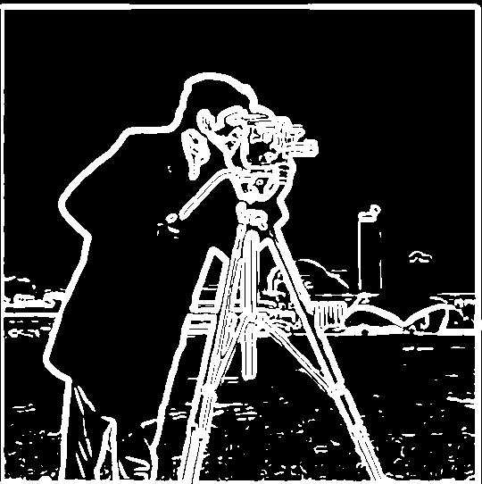
The gradient magnitude combines derivatives Dx and Dy to analyze edge strength in any direction: sqrt(dx² + dy²). In the gradient magnitude output image, edges are represented by bright white pixels, whereas flatter areas are represented in dark pixels. To create a binary edge image, each pixel above a tested gradient magnitude threshold is treated as an edge. Below show the results of testing thresholds from 0.05 to 0.3.
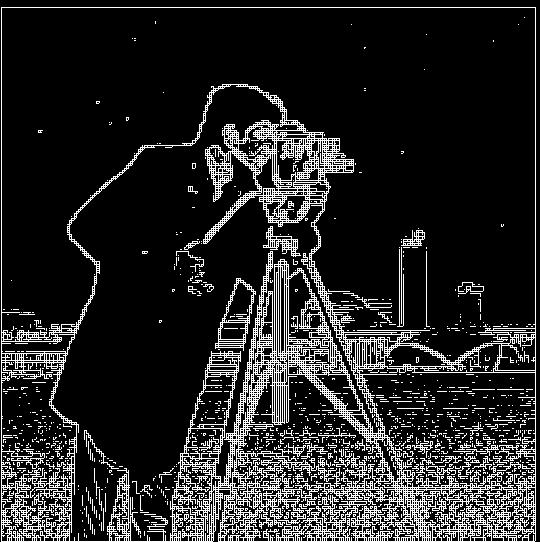
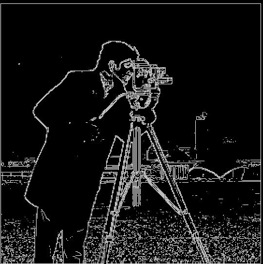
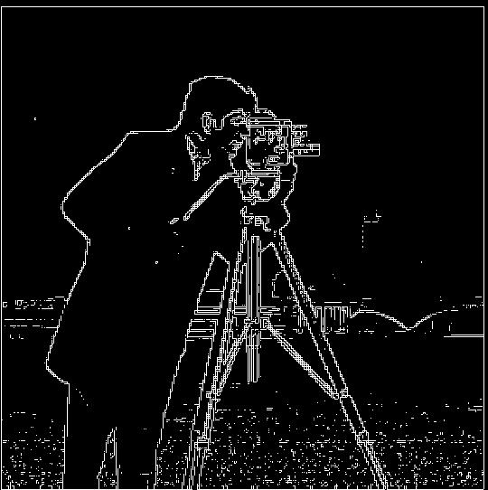
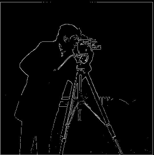
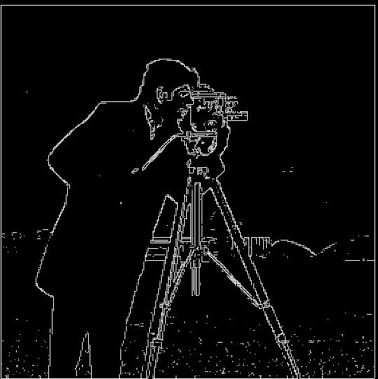
In the tested thresholds from 0.05 to 0.3, 0.2 was the best compromise, where the outline of the man's jacket and face, camera, tripod, and some of the skyline are visible, while minimal noise is shown in the grass and sky. Meanwhile, the 0.05, 0.1, and 0.15 images show heavier noise in the grass; 0.3 retains minimal background details; and 0.05 creates less visibility around the man's face and the camera.
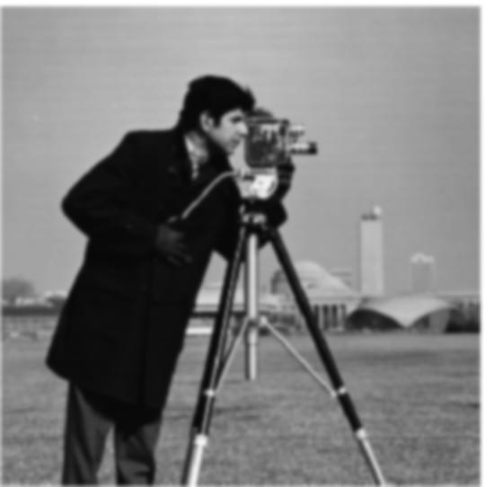
To fix the blurry results from Part 1.2, I first blurred the image with a Gaussian filter to remove high-frequency texture. Since blurring spreads each edge across its neighboring pixels, the brightness step between these neighboring pixels gets smaller. The maximum gradient magnitude dropped from 0.85 to 0.18, so with the Gaussian blur, I tested thresholds 0.02 to 0.08.
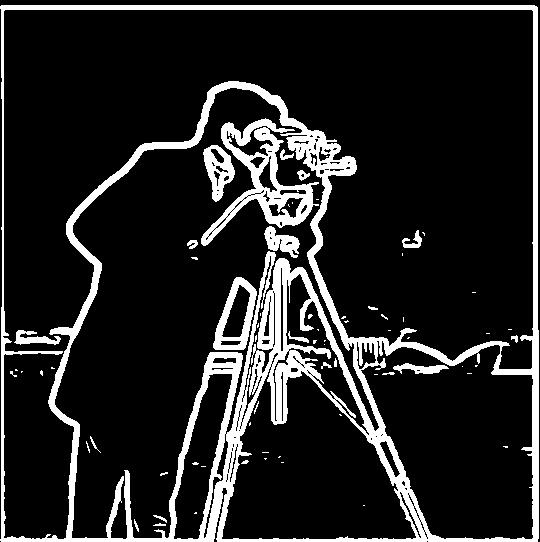
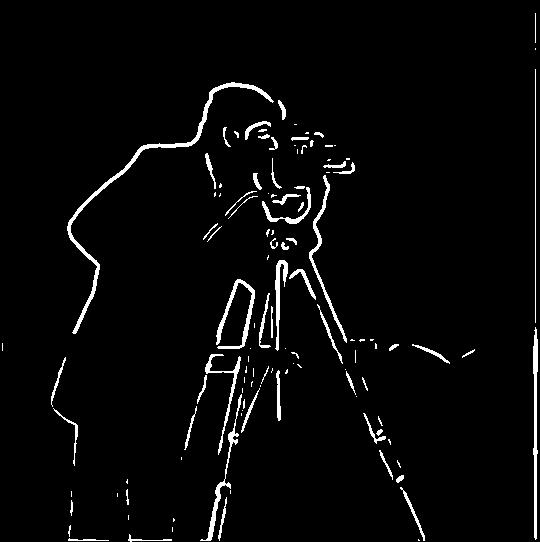
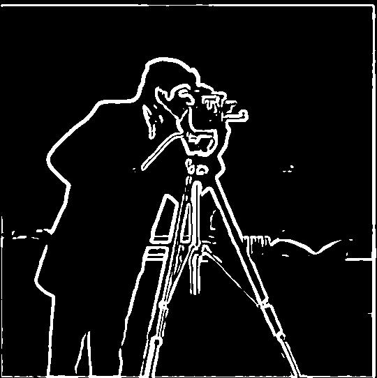
In the tested thresholds 0.02, 0.03, 0.05, and 0.08, 0.05 was the best image since it retained sufficient edge details from the man's face, jacket, and camera with a bit of detail left in the background, yet the lines weren't too thick or too thin for the image to be unclear. The 0.02 and 0.03 images on the other hand, have very thick lines, which obscure parts of the image and introduce a bit of noise with the grass and sky areas. The 0.08 image, however, is quite thin and loses details, with incomplete edges in the man's legs and the camera. A tradeoff of the selected 0.05 image as well as the 0.08 image is that both lack detail in the skyline.
With the Gaussian filter, the edges turn from thin and jagged to thick, smooth, and defined, making it easier to detect detailed objects, like the tripod legs. Some of the noise is lost as well in the grass area. However, a tradeoff is that some of the fine details are lost, like the man's facial features (specifically his ear, nose, and mouth).
Instead of applying a Gaussian filter and then differentiating it, in Method 2 we use a single convolution by creating a derivative of gaussian filters.
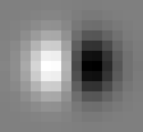
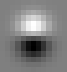
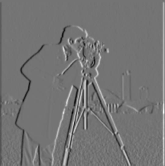
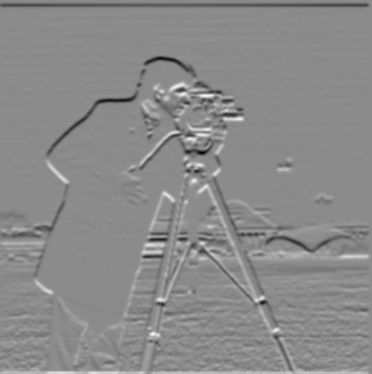
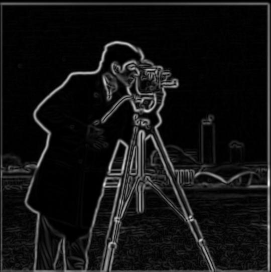
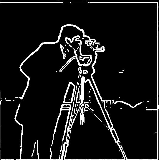
Method 1 and Method 2 produce the same result visually with the gradient magnitudes and binarized edge images.
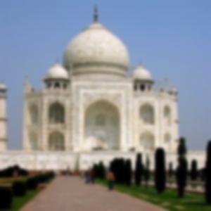
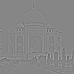
Gaussian blurs are low-pass filters that only keep the low frequencies of an image, creating a blurred effect. Therefore, if we subtract the low frequencies from an original sharp image, we are left with the high frequencies, which include edges and details. An unsharp mask helps take a blurry image and adds back the high frequencies to create a sharpened look. In the sample images below, you can see the original Taj Mahal image, along with various versions of it (with low frequencies only, high frequencies only, and varying levels of sharpening with the unsharp mask).
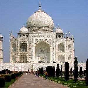
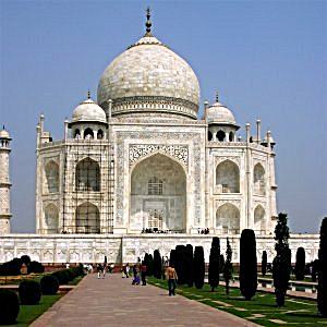
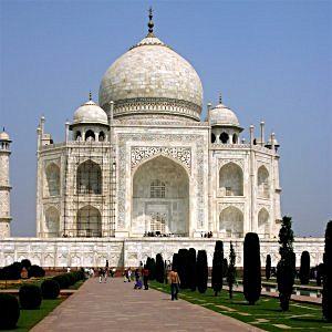
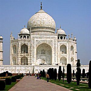
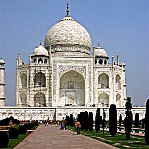
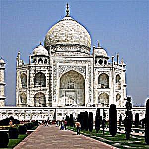
For the Taj Mahal image, the best sharpening factor is α = 1, where fine details like the outlines of bricks on the dome, tourists, and grass are clearly visible, yet noise is relatively low. In contrast, at α = 0.5, noise is still low but some details are still a bit fuzzy, such as the intricate carvings and brick outlines on the Taj Mahal. At α = 2 and 5, the noise greatly increases in the sky and on the building, making the image look unrealistically crisp with heavy edges.
In the experiments below, similarly, α = 1 is the best balance between noise and detail. For the tested images, when using a sharpening factor greater than α = 1, noise in large background areas such as the sky tend to increase greatly along with overly crisp details. For α = 0.5, noise is low, but some details are still fuzzy.
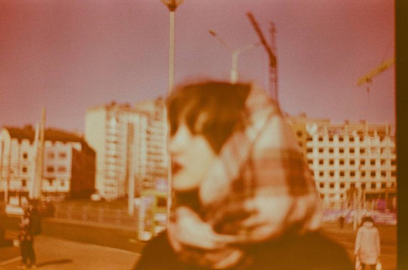
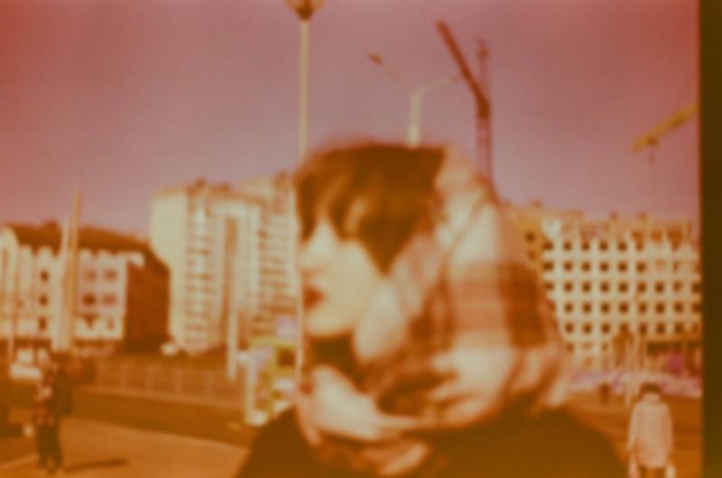
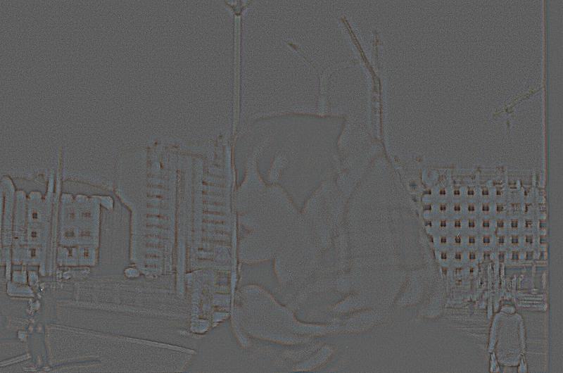
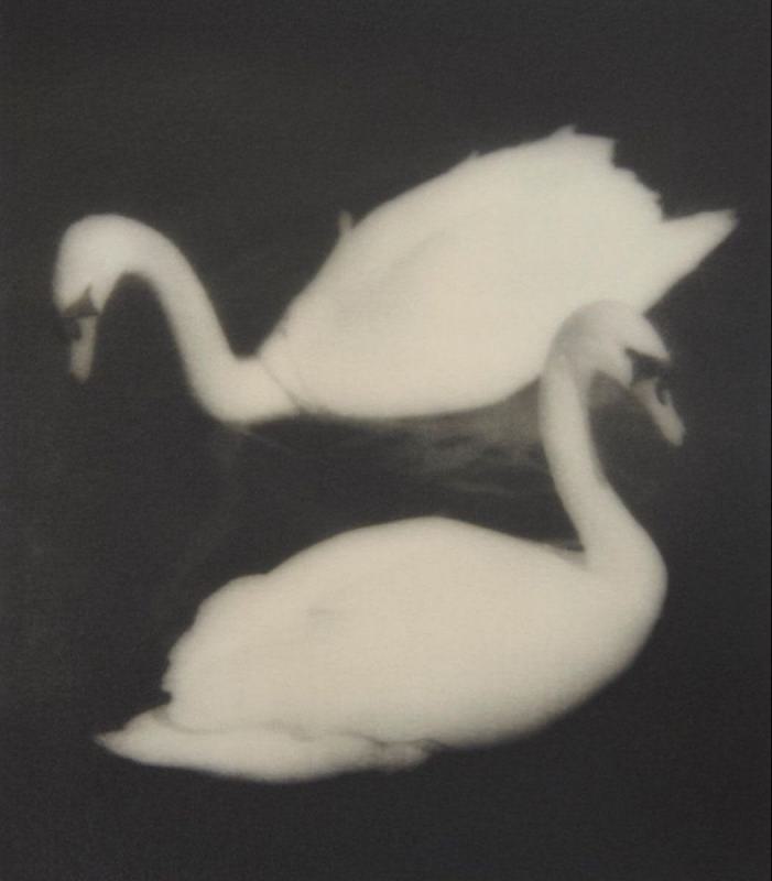
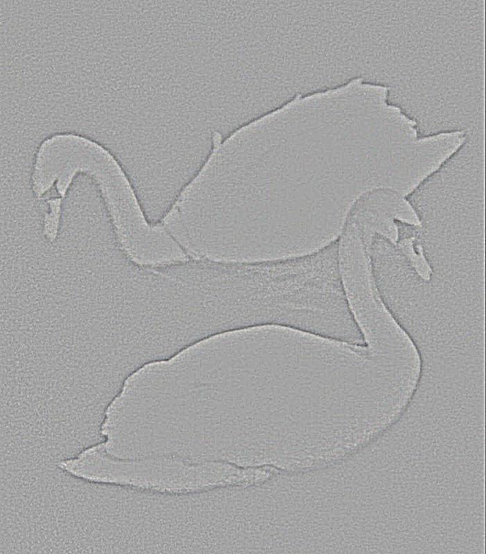
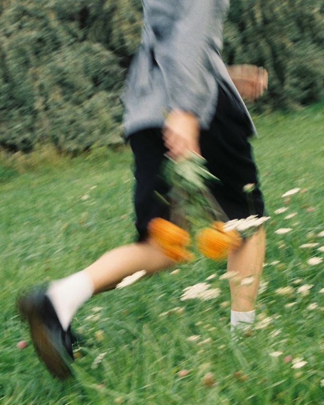
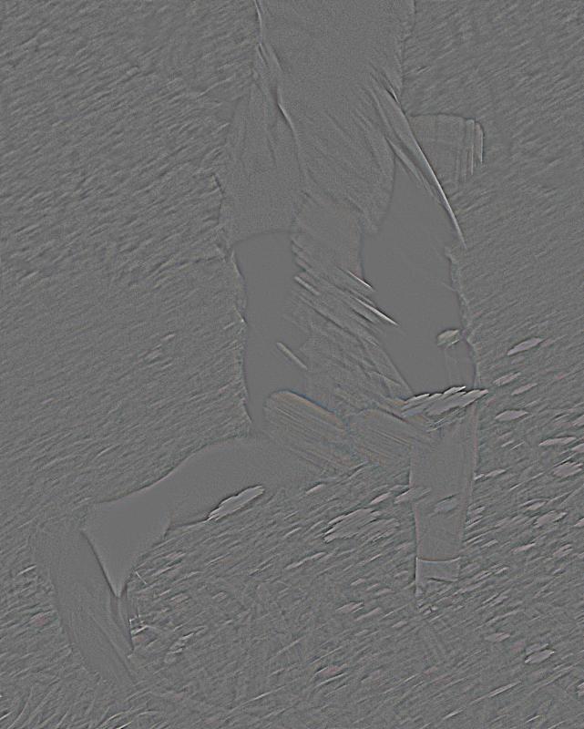
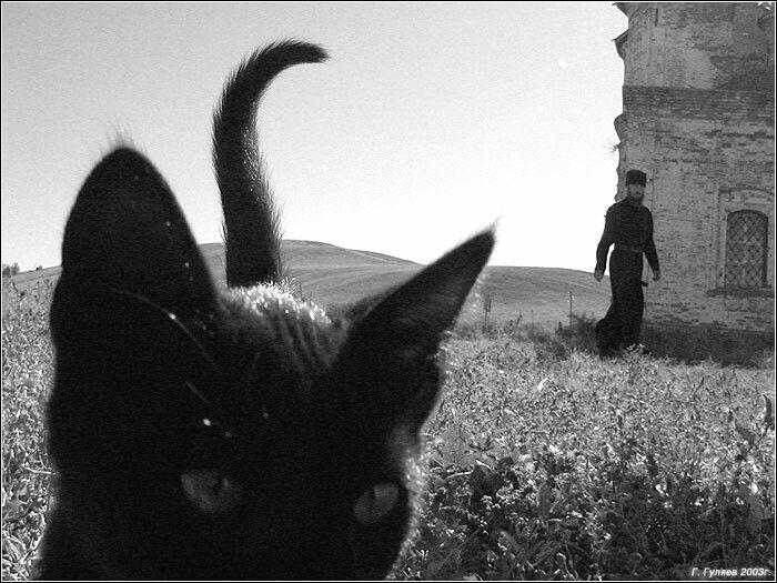
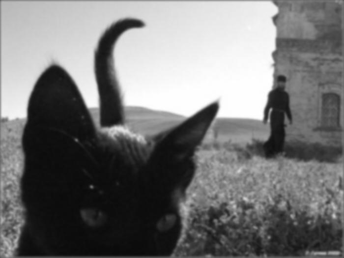
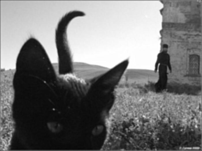
After applying the unsharp mask, the resharpened cat is clearer than the blurred version, but not all of the original fine details are recovered. This is especially visible at the top of the cat's head and its tail, which originally had very fine hair details visible. This is because the unsharp mask only amplifies high frequencies that were retained after the Gaussian filter was applied, leaving out some high frequencies from the original image.
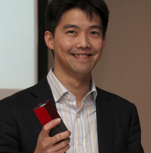
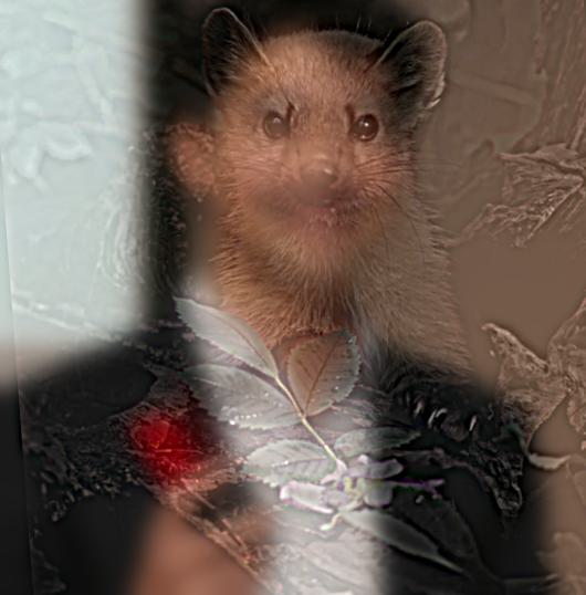
Hybrid images combine two images by combining the high frequencies from one image and the low frequencies from another image. This creates an optical illusion, where if you stand close to the hybrid image, it looks like the high frequency image, and if you stand far away, it looks like the low frequency image. The starter code helps align the two images with rotations, shifts, and scaling, given two user-made selections of alignment points on each image. To create the low frequency image, you can apply a Gaussian filter to one image, and to create the high frequency image, you can subtract the Gaussian-filtered version of itself from itself. After adding the two, the resulting hybrid image is cropped since the image that was rotated results in a black padding near the borders.
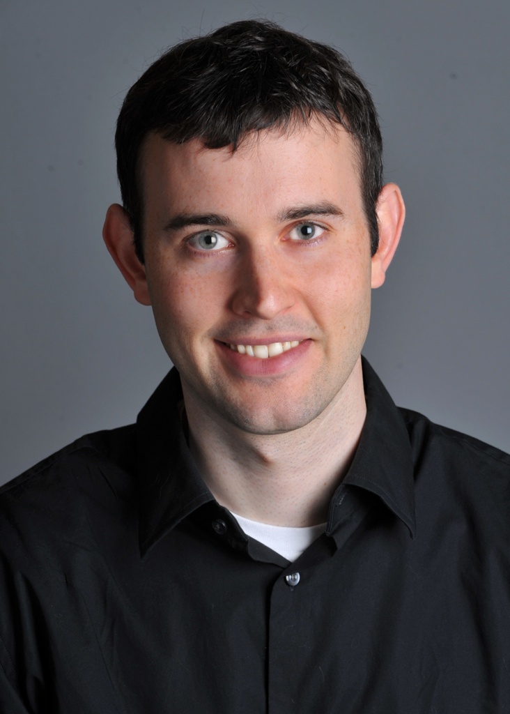
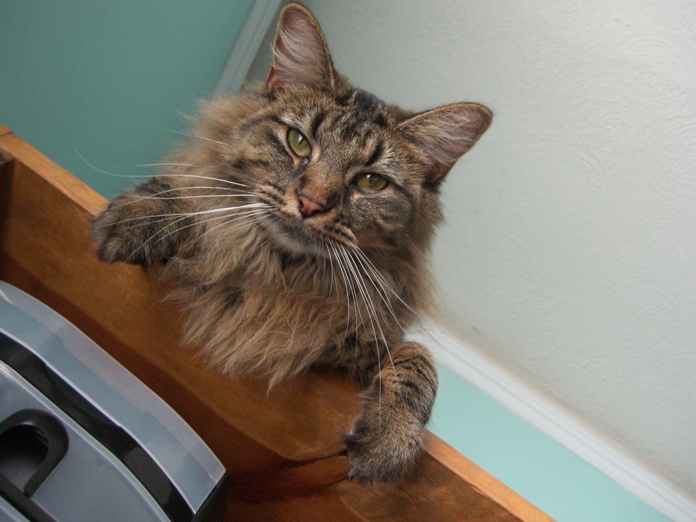
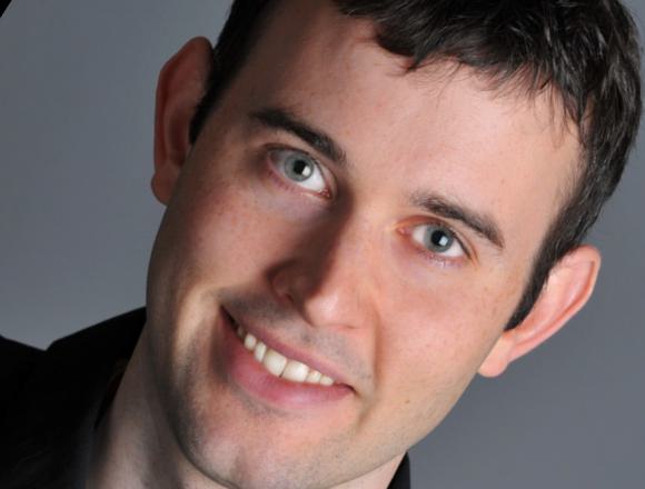
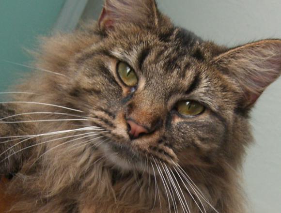
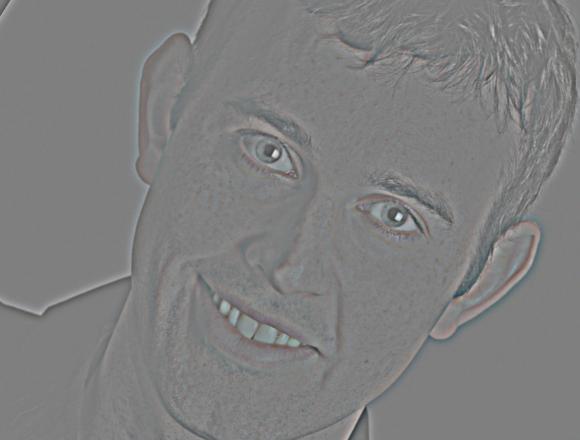
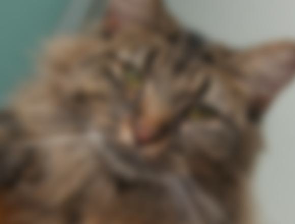
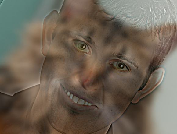
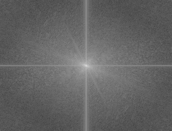
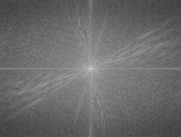
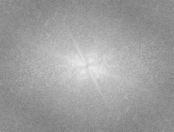
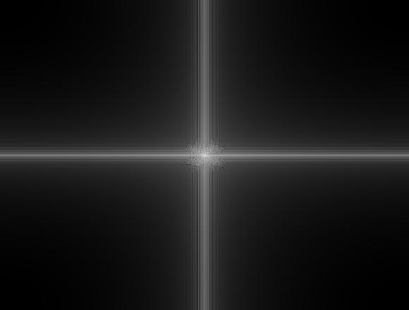
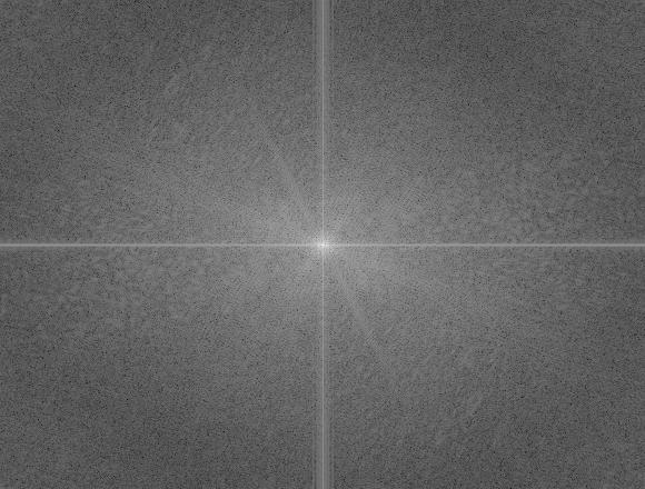
The Fourier transforms of each of the above images represent the image in the frequency domain. When applying the low-pass filter, the brightness is concentrated in the middle of the image, whereas when applying the high-pass filter, the brightness is concentrated in the outer regions of the image. The hybrid image's fourier transform combines the center brightness of the low-pass filtered image and the outer brightness of the high-pass filtered image.
In terms of choosing the cutoff frequencies, σ2 = 8 allowed Nutmeg's general shape, coloring, and darker fur markings to remain visible, while finer details like her whiskers and fur texture were removed. For σ1 = 4, Derek's facial features like his eyes and smile were able to be seen. A smaller σ2 let too much of Nutmeg's detail through, so she competed with Derek up close, and a larger σ1 kept Derek visible even from far away. With these cutoff frequencies, the hybrid image combines Derek and Nutmeg's features by retaining general shapes from one and finer details from the other, so that they're not competing for visibility.
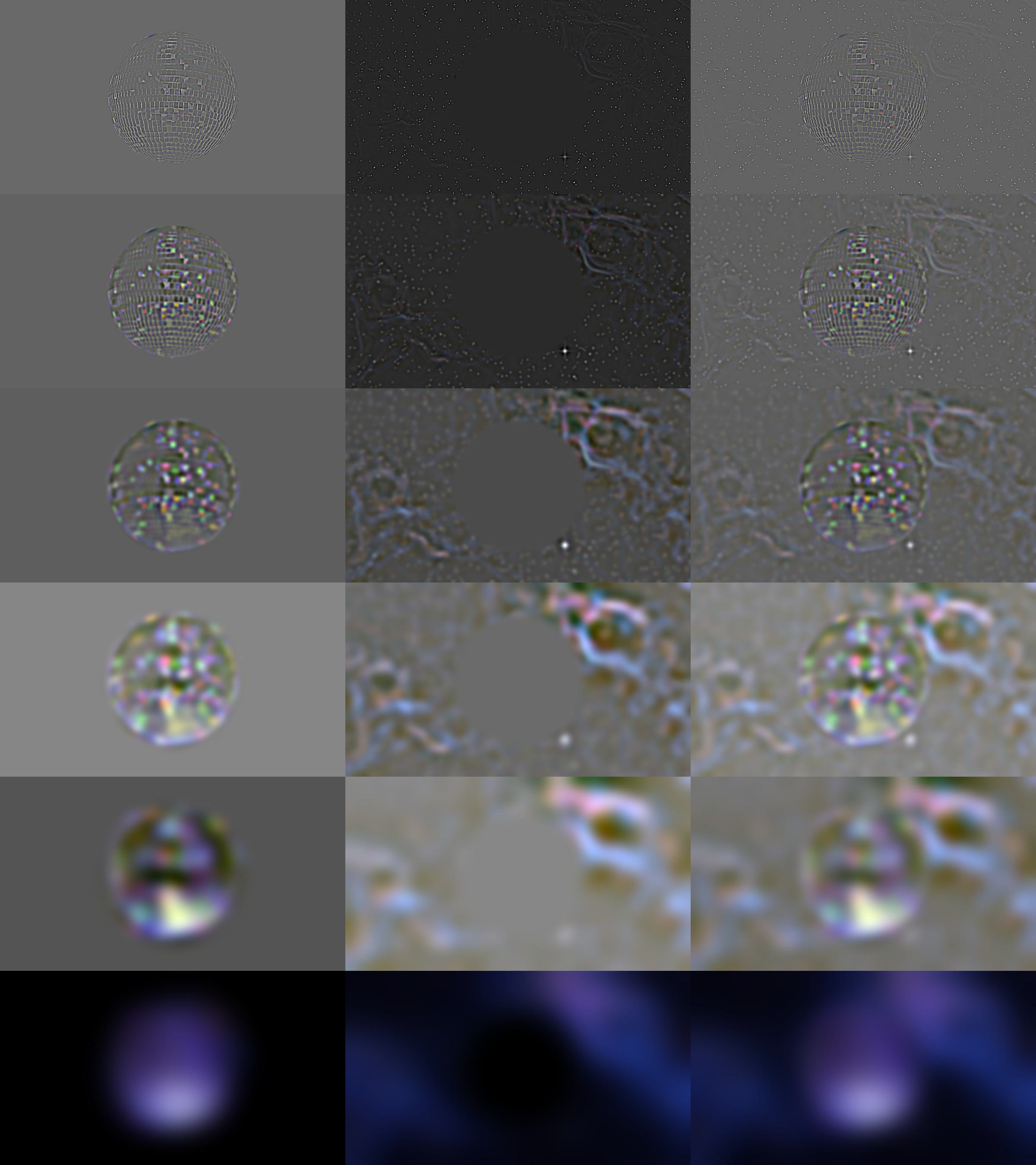
Gaussian and Laplacian stacks are used to create a multi-resolution blend of two images. In a Gaussian stack, an image is progressively blurred using an increasing σ, or value of Gaussian blur, at a fixed dimension, in contrast to a Gaussian pyramid which downsamples the image. Laplacian stacks subtract the difference between neighboring Gaussian levels, storing fine details at top layers, edges and other basic features at middle layers, and large background areas at bottom layers.





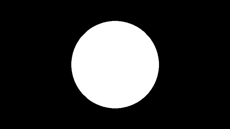
This mask represents how the two images should be blended: how much of each image should be shown and how much of a gradient there should be / the smoothness of the blend. In the above example, the white part of the mask represents the apple, and the black part of the mask represents the orange.
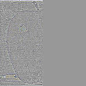
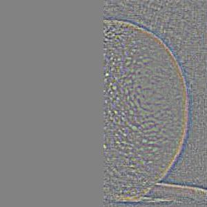
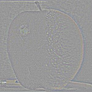
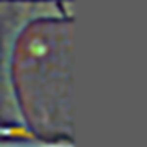
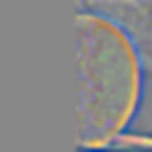
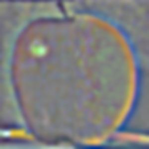
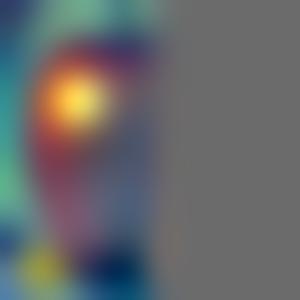
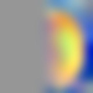
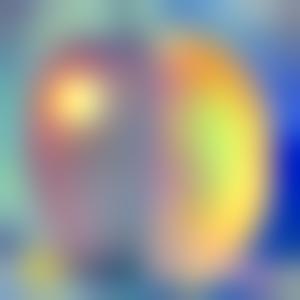
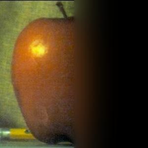
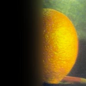
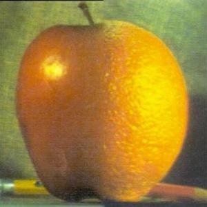
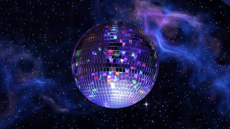
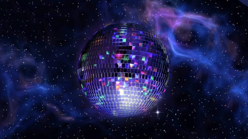
By combining the above Gaussian and Laplacian stacks, we can recreate Szeliski Figure 3.42 by sampling the apple, orange, and blended photos at levels 0, 2, and 4, additionally demonstrating the effects of the binary blend mask.

The most important thing I learned is that images can be represented as frequencies. In each of the different techniques we explored, from blurring to sharpening and creating hybrid images, we separated and recombined images based on their low and high frequencies.